An Extension to Basic ME Tableaux (1) 11ai Example Given: 1. Rx Px, - PowerPoint PPT Presentation

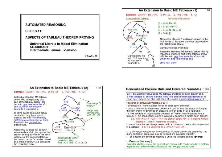
An Extension to Basic ME Tableaux (1) 11ai Example Given: 1. Rx ∨ ¬Px, 2. Px ∨ Q, 3. ¬Ra ∨ ¬Rb, 4. ¬Q Standard ME Tableau Resolution Refutation (5 = 2+1): Rx ∨ Q AUTOMATED REASONING (6 = 5+3): ¬Rb ∨ Q Q Px1 ⇒ Pa (7 = 6+5): Q ∨ Q ⇒ Q SLIDES 11: ¬Q (9 = 8+4): [ ] Rx2=>Rx1 ¬Px2 ASPECTS OF TABLEAU THEOREM PROVING ⇒ Ra x2==x1 Notice that clauses 5 and 6 correspond to the leaf literals of the open branches after each of Universal Literals in Model Elimination ¬Ra ¬Rb the first 2 steps of ME. KE-tableaux x1==a Comparing step 3 with ME: Intermediate Lemma Extension Instead of standard ME tableau below ¬Rb try Rb ¬Pb repeating enclosed part of the tableau below Cannot unify Rb KB-AR - 09 ¬Rb but with new free variables x3 and x4, with Rx2 here as Q which will bind to b instead of a. Pb x2 has been (See next slide) bound to a. ¬Q An Extension to Basic ME Tableaux (2) 11aii Generalised Closure Rule and Universal Variables 11aiii Example Given: 1. Rx ∨ ¬Px, 2. Px ∨ Q, 3. ¬Ra ∨ ¬Rb, 4. ¬Q Let T be a partially developed ME tableau and B be an open branch of T. If free variable x1 occurs in some literal in B and all other occurrences of x1 Instead of standard ME tableau in an open branch are also in B, then x1 is called a universal variable in T . below ¬Rb try repeating blue Q** part of the tableau below ¬Rb Px1 Features of Universal Variables in T: ¬Q Can merge Q but with new free variables x3 • bindings to x1 cannot affect literals in other open branches; with Q** and x4, which will become Rx2 ⇒ Rx1 ¬Px2 • once a free variable becomes universal it cannot lose this status as long as bound to b instead of a. ⇒ Ra x1==x2 Merge step the convention for bindings on closure given on Slide 11av is followed ; In some cases can avoid actual corresponds • a free variable x1 might not be universal in T when first introduced into a to Q ∨ Q ⇒ Q ¬Ra ¬Rb duplication. e.g. here would tableau T, but can become so if x1 eventually occurs in a single open branch; x1==a close at the leaf ¬Rb (implicitly e.g. in S ∨ P(x1,y) ∨ Q(x1) ∨ R if the branch below P(x1,y) is closed without matching a second copy of Rx2). Px3 ⇒ Pb binding x1, then x1 becomes universal. Q Results in the generalised • some variables are always universal in a clause and hence also when used closure rule. in a tableau e.g. y is universal in S ∨ P(x,y) ∨ Q(x) ∨ R ; Rx4 ⇒ Rx3 ¬Px4 ¬Q x4==x3 Notice that x2 does not occur in x3==b • a Universal variable can be treated as if it were universally quantified - as any open branch to the right of the many (different) copies as may be needed are available implicitly; branch ending at ¬Rb. In the fresh • as a result any bindings made to a universal variable can be ignored . instance of the enclosed tableau corresponds to the the branch below Q can be closed resolution step • Exercise (Not easy!) : by a merge with Q**, so simulating Rx1 ∨ Q + ¬Rb ∨ Q ⇒ Q ∨ Q the resolution proof. Consider whether use of the generalised closure rule can be used in a tableau together with either the (re-use) and/or the (merge) closure rules.

11av An Important Criterion 11aiv Example Revisited In Example A , to close at (1), it is important to introduce instance P(x2) of the implicit ∀ x.P(x). Rx ∨ ¬Px, Px ∨ Q, ¬Ra ∨ ¬Rb, ¬Q x1 not A Q Px1 Px1 in If instead x2 and x1 were simply bound to each other, (∀ x.P(x)) In Px ∨ Q x is universal. The clause Px1 ∨ Q is used (∀ x.P(x)) here then x1 would be propagated to both Rx2 and Sx2 ∀ x.P(x) ∨ ∀ ∨ Q . ∨ ¬Q in the tableau as if it were ∀ ∀ ∨ and x1 would lose its universal status. ¬Px2 At closure (1) use instance P(x2) of ∀ x.P(x). ¬Px2 Rx2 Rx2 Sx2 (∀ x.R(x)) (1) In Example B, when closing at (2) it is important to Rx2 becomes universal and is treated as ∀ x.R(x). (1) introduce instance ¬Px1 of implicit ∀ x.¬P(x). At closure (2) use instance R(a) of ∀ x.R(x). Otherwise x2 and x1 would be bound to each other ¬Ra ¬Rb and x2 would lose its universal status, which would At closure (3) use instance R(b) of ∀ x.R(x). (2) (3) affect the literal Rx2 as well. B S(x1) P(x1) None of the bindings made affects the branch beneath Q, since the universal These observations lead to the following convention variables do not appear in it. That branch only needs to be completed once. which will guarantee universal variables remain so. ¬Py2 Rx2 ( ∀ x.R(x)) What if clause Rx ∨ ¬Px happened to be Rx ∨ ¬Px ∨ Sx? y2==x1 In making a closure that involves at least one Variable x in {Rx ∨ ¬Px ∨ Sx is not universal, so it is important not to attempt ¬Px2 x2 not ¬Rx2 universal variable always introduce an instance to bind x1 to x2 at closure (1), as x1 would then lose its universal status. ( ∀ x.¬P(x) in of the universal variable to make the closure. Instead, use a fresh instance of x1. (2) here Normal Form Representation of a Partial Tableau 11avi 11avii Generalised Closure Rule: Given (1) ¬P(a) ∨∀ z.¬A(b,z) ; (2) ¬R(c) ∨ ¬A(c,c) (3) ∀ x.A(x,y) ∨ B(y) (4) ¬A(x,y) ∨ P(x) ∨ R(y) The slides 11ai - 11avi illustrate and explain an extension for ME-tableaux called the generalised closure rule , which uses the concept of a universal variable . For the simplest Consider the tableau after closure (1) (above the case, let C be a clause in which variable u occurs in exactly one literal L. u is called a wavy line). The open branches ≡ universal variable . The quantifier for this variable could (implicitly) be distributed across to ∀ y1 [( ∀ x.A(x,y1) ∧ ( ∀ x.P(x) ∨ R(y1))) ∨ B(y1)] (*) ≡ L. When the clause is developed, one can treat L as if it were ∀ u.L, implicitly including in ∀ y[( ∀ x.A(x,y) ∧∀ x.P(x)) ∨ ( ∀ x.A(x,y) ∧ R(y)) ∨ B(y)] ∀ x.A(x,y1) the tableau branch containing L several copies of L, each with a fresh free variable for u. B(y1) (Any non-universal variables in L would each have the same free variables substituted in all copies.) The effect is that bindings to u can be ignored since there are available enough Before treating variables as universal, the R(y2) copies for each different binding, giving rise to the generalised closure rule . This rule states expression would have been: ¬ A(x1,y2) ⇒ P(x1) that in any closure step involving a universal variable u possible bindings to u can be ∀ y1 ∀ x1[(A(x1,y1) ∧ (P(x1) ∨ R(y1)) ∨ B(y1)] ≡ y2==y1 (∀ x.P(x)) R(y1) ignored. (1) ∀ y [ ∀ x[A(x,y) ∧ (P(x) ∨ R(y)) ] ∨ B(y)] ≡ (∗) Effect is to maximally distribute ∀ . e.g. if L is P(v,u), and u is universal but v is not, then L is regarded as if it were ∀ u.P(v,u) and can be copied in the tableau as P(v1,u1), P(v1,u2), giving the possibility of closure with ¬P(a) ¬P(a,b) ∨ ¬P(a,c), for example. If L is part of a clause L ∨ Q(w), the duplication treats the Variables x and z in clauses (3)/ (1) are universal. Notice x1 becomes universal and y1 is not clause as having the more general (nnf) form (P(v,u1) ∧ P(v,u2)) ∨ Q(w). ∀ z.¬A(b,z) universal. Can ``forget’’ the bindings to universal ¬A(c,c) More generally, let T be a partially developed ME tableau and B be an open branch of T. (**) variables (they are not shown). Thus instances ¬R(c) If free variable x1 occurs in some literal in B and all other occurrences of x1 in an open A(x3,y1) and A(b,z3) are unified at (**) leaving y1 y1==c branch are also in B, then x1 is called a universal variable in T. unbound. It is bound to c at (***). After the closures (***) the remaining open branch contains B(c). Notice (Note: in the Chapter" notes, the generalised closure rule was also called generalised ancestor B(c) can be derived B(c) from (*), (1) and (2). resolution.)