An Example Blackjack: Goal is to obtain cards whose sum is as great - PowerPoint PPT Presentation

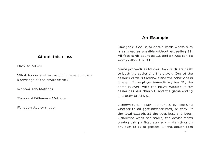
An Example Blackjack: Goal is to obtain cards whose sum is as great as possible without exceeding 21. All face cards count as 10, and an Ace can be About this class worth either 1 or 11. Back to MDPs Game proceeds as follows: two cards are dealt to both the dealer and the player. One of the What happens when we don’t have complete dealer’s cards is facedown and the other one is knowledge of the environment? faceup. If the player immediately has 21, the game is over, with the player winning if the Monte-Carlo Methods dealer has less than 21, and the game ending in a draw otherwise. Temporal Di ff erence Methods Otherwise, the player continues by choosing Function Approximation whether to hit (get another card) or stick . If the total exceeds 21 she goes bust and loses. Otherwise when she sticks, the dealer starts playing using a fixed strategy – she sticks on any sum of 17 or greater. IF the dealer goes 1 2

bust the player wins, otherwise the winner is (b) Presence of a usable ace (that doesn’t determined by who has a sum closer to 21. have to be counted as 1) (c) Dealer’s faceup card Assume cards are dealt from an infinite deck (i.e. with replacement) Total of 200 states Formulation as an MDP: Problem: find the value function for a policy that always hits unless the current total is 20 1. Episodic, undiscounted or 21. 2. Rewards of +1 (winning), 0 (draw), -1 Suppose we wanted to apply a dynamic pro- (losing) gramming method. We would need to figure out all the transition and reward probabiliies! This is not easy to do for a problem like this. 3. Actions: hit, stick Monte Carlo methods can work with sample episodes alone! 4. State space: determined by (a) Player’s current sum (12-21, because It’s easy to generate sample episodes for our player always hits below 12) Blackjack example.

The Absence of a Transition Model We now want to estimate action values rather than state values. So estimate Q π ( s, a ) In first-visit MC, to evaluate a policy π , we re- Problem? If π is deterministic, we’ll never learn peatedly generate episodes using π , and then the values of taking di ff erent actions in partic- store the return achieved following the first oc- ular states... currence of each state in the episode. Then, averaging these over many simulations gives us Must maintain exploration. This is sometimes the expected value of each state under policy dealt with through the concept of exploring π starts – randomize over all actions at the first state in each episode. Somewhat problematic assumption – nature won’t always be so kind – but it should work OK for Blackjack 3

Coming Up With Better Policies We can interleave policy evaluation with policy improvement as before. � * V * 21 STICK 20 E → Q π 0 I E → · · · I → π ∗ E → Q ∗ 19 π 0 → π 1 − − − − − 1 Usable 18 + 1 2 17 ace 16 � 1 15 A HIT 14 13 12 We’ve just figured out how to do policy eval- 11 A 2 3 4 5 6 7 8 9 10 12 1 0 uation. 21 20 19 Player sum STICK 1 No 18 2 17 usable Policy improvement is even easier because now 16 Player sum 15 ace A HIT 14 13 we have the direct expected rewards for each D e a 12 l e r 11 s h o action in each state Q ( s, a ) so just pick the A 2 3 4 5 6 7 8 9 w 10 i n 12 g Dealer showing 1 0 best action among these The optimal policy for Blackjack: 4

On-Policy Learning On-policy methods attempt to evaluate the same policy that is being used to make de- cisions Get rid of the assumption of exploring starts. Now use an ǫ -greedy method where some ǫ pro- portion of the time you don’t take the greedy the best one can do with general strategies in action, but instead take a random action the new environment is the same as the best one could do with ǫ -greedy strategies in the Soft policies: all actions have non-zero proba- old environment. bilities of being selected in all states For any ǫ -soft policy π , any ǫ -greedy strategy with respect to Q π is guaranteed to be an im- provement over π . If we move the ǫ -greedy requirement inside the environment, so that we say nature randomizes your action 1 − ǫ proportion of the time, then 5

Temporal-Di ff erence Learning What is MC estimation doing? Adaptive Dynamic Programming V ( s t ) ← (1 − α t ) V ( s t ) + α t R t Simple idea – take actions in the environment where R t is the return received following being (follow some strategy like ǫ -greedy with re- in state s t . spect to your current belief about what the value function is) and update your transition Suppose we switch to a constant step-size α and reward models according to observations. (this is a trick often used in nonstationary en- Then update your value function by doing full vironments) dynamic programming on your current believed model. TD methods basically bootstrap o ff of exist- ing estimates instead of waiting for the whole In some sense this does as well as possible, reward sequence R to materialize subject to the agent’s ability to learn the tran- sition model. But it is highly impractical for V ( s t ) ← (1 − α ) V ( s t ) + α [ r t +1 + γ V ( s t +1 )] anything with a big state space (Backgammon (based on actual observed reward and new state) has 10 50 states) This target uses the current value as an es- timate of V whereas the Monte Carlo target 6 7

Q-Learning: A Model-Free Approach Even without a model of the environment, you can learn e ff ectively. Q-learning is conceptually similar to TD-learning, but uses the Q function uses the sample reward as an estimate of the instead of the value function expected reward 1. In state s , choose some action a using pol- If we actually want to converge to the opti- icy derived from current Q (for example, mal policy, the decision-making policy must ǫ -greedy), resulting in state s ′ with reward be GLIE (greedy in the limit of infinite explo- r . ration) – that is, it must become more and more likely to take the greedy action, so that 2. Update: we don’t end up with faulty estimates (this Q ( s ′ , a ′ )) Q ( s, a ) ← (1 − α ) Q ( s, a )+ α ( r + γ max problem can be exacerbated by the fact that a ′ we’re bootstrapping) You don’t need a model for either learning or action selection! As environments become more complex, using a model can help more (anecdotally) 8

Suppose our linear function predicts V θ ( s ) and Generalization in Reinforcement we actually would “like” it to have predicted Learning something else, say v . Define the error as E ( s ) = ( V θ ( s ) − v ) 2 / 2. Then the update rule So far, we’ve thought of Q functions and utility is: functions as being represented by tables θ i ← θ i − α∂ E ( s ) ∂θ i Question: can we parameterize the state space = θ i + α ( v − V θ ( s )) ∂ V θ ( s ) so that we can learn (for example) a linear ∂θ i function of the parameterization? If we look at the TD-learning updates in this framework, we see that we essentially replace V θ ( s ) = θ 1 f 1 ( s ) + θ 2 f 2 ( s ) + · · · + θ n f n ( s ) what we’d “like” it to be with the learned backup (sum of the reward and the value func- tion of the next state: Monte Carlo methods: We obtain sample of θ i ← θ i + α [ R ( s ) + γ V θ ( s ′ ) − V θ ( s )] ∂ V θ ( s ) V ( s ) and then learn the θ ’s to minimize squared ∂θ i error. This can be shown to converge to the closest In general, often makes more sense to use an function to the true function when linear func- online procedure, like the Widrow-Ho ff rule: tion approximators are used, but it’s not clear 9

how good a linear function will be at approxi- mating non-linear functions in general, and all bets on convergence are o ff when we move to non-linear spaces. The power of function approximation: allows you to generalize to values of states you haven’t yet seen! In backgammon, Tesauro constructed a player as good as the best humans although it only examined one out of every 10 44 possible states. Caveat: this is one of the few successes that has been achieved with function approximation and RL. Most of the time it’s hard to get a good parameterization and get it to work.