An Analysis of Graph Cut Size for Transductive Learning Steve - PowerPoint PPT Presentation
An Analysis of Graph Cut Size for Transductive Learning Steve Hanneke Machine Learning Department Carnegie Mellon University 1 Outline Transductive Learning with Graphs Error Bounds for Transductive Learning Error Bounds Based
An Analysis of Graph Cut Size for Transductive Learning Steve Hanneke Machine Learning Department Carnegie Mellon University
1 Outline • Transductive Learning with Graphs • Error Bounds for Transductive Learning • Error Bounds Based on Cut Size MACHINE LEARNING DEPARTMENT
2 Transductive Learning Classifier Predictions Labeled Labeled Unlabeled Training Training Test Data Predictions Data Data iid Random Split Unlabeled iid Distribution Test Data Data Inductive Learning Transductive Learning MACHINE LEARNING DEPARTMENT
3 Vertex Labeling in Graphs • G=(V,E) connected unweighted undirected graph. |V|=n. (see the paper for weighted graphs). • Each vertex is assigned to exactly one of k classes {1,2,…,k} (target labels). • The labels of some (random) subset of n � vertices are revealed to us. (training set) • Task: Label the remaining (test) vertices to (mostly) agree with the target labels. MACHINE LEARNING DEPARTMENT
4 Example: Data with Similarity 2 2 2 1 3 1 • Vertices are examples in an instance space and edges exist between similar examples. • Several clustering algorithms use this representation. • Useful for digit recognition, document classification, several UCI datasets,… MACHINE LEARNING DEPARTMENT
5 Example: Social Networks 2 2 2 1 1 3 • Vertices are high school students, edges represent friendship, labels represent which after-school activity the student participates in (1=football, 2=band, 3=math club, …). MACHINE LEARNING DEPARTMENT
6 Adjacency • Observation: Friends tend to be in the same after-school activities. ? = 2 2 2 1 1 3 • More generally, it is often reasonable to believe adjacent vertices are usually classified the same. • This leads naturally to a learning bias. MACHINE LEARNING DEPARTMENT
7 Cut Size • For a labeling h of the vertices in G, define the Cut Size , denoted c(h), as the number of edges in G s.t. the incident vertices have different labels (according to h). 2 2 2 1 1 3 Example: Cut Size 2 MACHINE LEARNING DEPARTMENT
8 Learning Algorithms • Several existing transductive algorithms are based on the idea of minimizing cut size in a graph representation of data (in addition to number of training errors, and other factors). • Mincut (Blum & Chawla, 2001) • Spectral Graph Transducer (Joachims, 2003) • Randomized Mincut (Blum et al., 2004) • others MACHINE LEARNING DEPARTMENT
9 Mincut (Blum & Chawla, 2001) • Find a labeling having smallest cut size of all labelings that respect the known labels of the training vertices. • Can be solved by reduction to multi- terminal minimum cut graph partitioning • Efficient for k=2. • Hard for k>2, but have good approximation algorithms MACHINE LEARNING DEPARTMENT
10 Error Bounds • For a labeling h, define and the fractions of training vertices and test vertices h makes mistakes on, respectively. (training & test error) • We would like a confidence bound of the form MACHINE LEARNING DEPARTMENT
11 Bounding a Single Labeling • Say a labeling h makes T total mistakes. The number of training mistakes is a hypergeometric random variable. • For a given confidence parameter δ , we can “invert” the hypergeometric to get MACHINE LEARNING DEPARTMENT
12 Bounding a Single Labeling • Single labeling bound: • We want a bound that holds simultaneously for all h. • We want it close to the single labeling bound for labelings with small cut size. MACHINE LEARNING DEPARTMENT
13 The PAC-MDL Perspective • Single labeling bound: • PAC-MDL (Blum & Langford, 2003): • where p( ⋅ ) is a probability distribution on labelings. (the proof is basically a union bound) • Call δ p(h) the “tightness” allocated to h. MACHINE LEARNING DEPARTMENT
14 The Structural Risk Trick δ H δ /(|E|+1) δ /(|E|+1) δ /(|E|+1) δ /(|E|+1) δ /(|E|+1) δ /(|E|+1) S 0 S 1 S 2 S 3 S c S |E| . . . . . . S c =labelings with cut size c. Split the labelings into |E|+1 sets by cut size and allocate δ /(|E|+1) total “tightness” to each set. MACHINE LEARNING DEPARTMENT
15 The Structural Risk Trick δ /(|E|+1) S c h c1 h c2 h c3 h c4 h ci h cSc Within each set S c , divide the δ /(|E|+1) tightness equally amongst the labelings. So each labeling receives tightness exactly . This is a valid δ p(h). MACHINE LEARNING DEPARTMENT
16 The Structural Risk Trick • We can immediately plug this tightness into the PAC-MDL bound to get that with probability at least 1- δ , every labeling h satisfies • This bound is fairly tight for small cut sizes. • But we can’t compute |S c |. We can upper bound |S c |, leading to a new bound that largely preserves the tightness for small cut sizes. MACHINE LEARNING DEPARTMENT
17 Bounding |S c | • Not many labelings have small cut size. • At most n 2 edges, so • But we can improve this with data- dependent quantities. MACHINE LEARNING DEPARTMENT
18 Minimum k-Cut Size • Define minimum k-cut size , denoted C(G), as minimum number of edges whose removal separates G into at least k disjoint components. • For a labeling h, with c=c(h), define the relative cut size of h MACHINE LEARNING DEPARTMENT
19 A Tighter Bound on |S c | • Lemma: For any non-negative integer c, |S c | � B( � (c)), where for ½ � � < n/(2k), • (see paper for the proof) • This is roughly like (kn) � (c) instead of (kn) c . MACHINE LEARNING DEPARTMENT
20 Error Bounds • |S c | � B( � (c)), so the “tightness” we allocate to any h with c(h)=c is at least • Theorem 1 (main result): With probability at least 1- δ , every labeling h satisfies (can be slightly improved: see the paper) MACHINE LEARNING DEPARTMENT
21 Error Bounds • Theorem 2 : With probability at least 1- δ , every h with ½ < � (h)<n/(2k) satisfies (overloading � (h)= � (c(h)) ) Something like training error + Proof uses result by Derbeko, et al. MACHINE LEARNING DEPARTMENT
22 Visualizing the Bounds n=10,000; n � =500; |E|=1,000,000; C(G)=10(k-1); δ =.01; no training errors. • Overall shapes are the same, so the loose bound can give some intuition. MACHINE LEARNING DEPARTMENT
23 Conclusions & Open Problems • This bound is not difficult to compute, it’s Free, and gives a nice guarantee for any algorithm that takes a graph representation as input and outputs a labeling of the vertices. • Can we extend this analysis to include information about class frequencies to specialize the bound for the Spectral Graph Transducer (Joachims, 2003)? MACHINE LEARNING DEPARTMENT
An Analysis of Graph Cut Size for Transductive Learning Steve Hanneke Questions? MACHINE LEARNING DEPARTMENT
Recommend
More recommend
Explore More Topics
Stay informed with curated content and fresh updates.
