An adaptive finite-volume method for a model of two-phase pedestrian - PowerPoint PPT Presentation

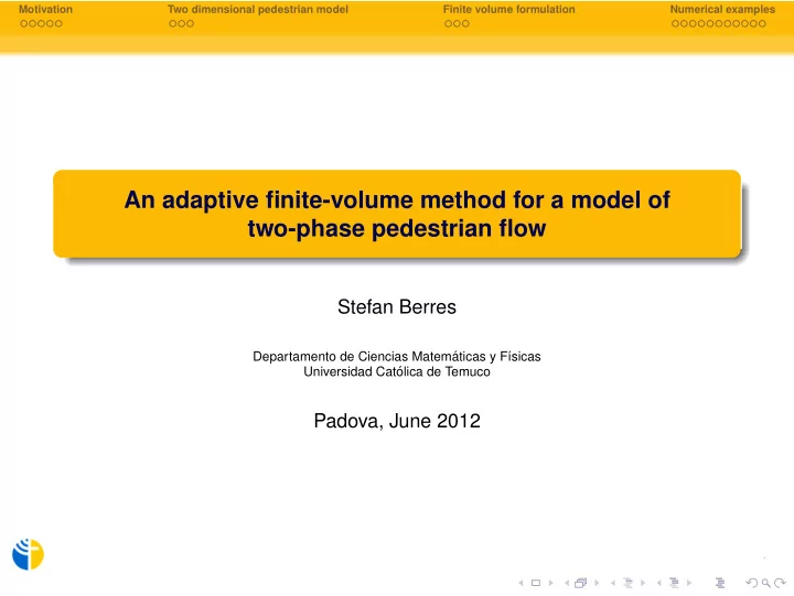
Motivation Two dimensional pedestrian model Finite volume formulation Numerical examples An adaptive finite-volume method for a model of two-phase pedestrian flow Stefan Berres Departamento de Ciencias Matem´ aticas y F´ ısicas Universidad Cat´ olica de Temuco Padova, June 2012

Motivation Two dimensional pedestrian model Finite volume formulation Numerical examples Outline Motivation 1 Elliptic region Polydisperse suspensions Bidisperse suspension Symmetric case δ = 1 , γ = − 1 Two dimensional pedestrian model 2 Modelling Model of Huges Finite volume formulation 3 A finite-volume formulation Multiresolution setting Numerical examples 4 Example 1: Flow towards exit targets Example 2: Battle of Agincourt Example 3: Countercurrent flow in a long channel Example 4: Countercurrent flow Example 5: Perpendicular flow with different velocity functions Example 6: Effect of diffusion and cross-diffusion

Motivation Two dimensional pedestrian model Finite volume formulation Numerical examples Elliptic region Systems with elliptic region We examine initial value problems for first-order systems ∂ t φ 1 + ∂ x f 1 ( φ 1 , φ 2 ) = 0 , (1.1) ∂ t φ 2 + ∂ x f 2 ( φ 1 , φ 2 ) = 0 , by applying multi-resolution schemes. We recall that the system (1.1) is called hyperbolic at a point ( φ 1 , φ 2 ) if the Jacobian J f of the flux vector f = ( f 1 , f 2 ) T , ∂ f 1 ∂ f 1   ∂φ 1 ∂φ 2 � J 11 � J 12   J f =  =:   J 21 J 22 ∂ f 2 ∂ f 2  ∂φ 1 ∂φ 2 has real eigenvalues, i.e., if the discriminant ( J 11 − J 22 ) 2 + 4 J 12 J 21 � � ∆( φ 1 , φ 2 ) := ( φ 1 , φ 2 ) (1.2) is positive, and strictly hyperbolic if these eigenvalues are moreover distinct. If J f ( φ 1 , φ 2 ) has a pair of complex conjugate eigenvalues (i.e., ∆( φ 1 , φ 2 ) < 0), then (1.1) is called elliptic at that point. The set of all elliptic points is called elliptic region.

Motivation Two dimensional pedestrian model Finite volume formulation Numerical examples Polydisperse suspensions Sedimentation of polydisperse suspensions Vector of unknows: solids concentrations Φ = ( φ 1 , φ 2 , . . . , φ N ) (1.3) Cumulative solids fraction φ := φ 1 + · · · + φ N , Hindered settling factor V ( 0 ) = 1 , V ′ ( φ ) ≤ 0 , V ( 1 ) = 0, e.g. � ( 1 − φ ) n − 2 if Φ ∈ D φ max , V ( φ ) = n > 2 . (1.4) 0 otherwise, Phase velocity of particle species i � � N d 2 � d 2 v i (Φ) = µ V ( φ ) i ( ̺ i − ̺ (Φ)) − m φ m ( ̺ m − ̺ (Φ)) , i = 1 , . . . , N . m = 1 (1.5) One-dimensional batch settling of a suspension ∂ t Φ + ∂ x f (Φ) = 0 , x ∈ ( 0 , L ) , t > 0 , (1.6) � T , � f (Φ) = f 1 (Φ) , . . . , f N (Φ) f i (Φ) = φ i v i (Φ) , i = 1 , . . . , N , Initial and zero-flux boundary conditions Φ( x , 0 ) = Φ 0 ( x ) , x ∈ [ 0 , L ] , f | x = 0 = f | x = L = 0 . (1.7)

Motivation Two dimensional pedestrian model Finite volume formulation Numerical examples Bidisperse suspension Model of bidisperse suspension For case N = 2, it is convenient to introduce the parameter ̺ 1 = ( ̺ 2 − ̺ r ) / ( ̺ 1 − ̺ r ) , and we set δ := δ 2 = d 2 1 / d 2 γ := ¯ ̺ 2 / ¯ 2 . � �� � f 1 ( φ 1 , φ 2 ) = φ 1 V ( φ 1 + φ 2 ) ( 1 − φ 1 )( 1 − φ 1 − γφ 2 ) − δφ 2 ( 1 − φ 2 ) γ − φ 1 , � � f 2 ( φ 1 , φ 2 ) = φ 2 V ( φ 1 + φ 2 ) δ ( 1 − φ 2 ) � ( 1 − φ 2 ) γ − φ 1 � − φ 1 ( 1 − φ 1 − γφ 2 ) . with δ ∈ ( 0 , 1 ] and hindered settling factor V ( φ ) ≥ 0, V ′ ( φ ) < 0 on [ 0 , φ max )

Motivation Two dimensional pedestrian model Finite volume formulation Numerical examples Symmetric case δ = 1 , γ = − 1 Symmetric case δ = 1 , γ = − 1 (B., B¨ urger, Kozakevicius 2009) For the symmetric case, where δ = 1 , γ = − 1, there are tangents on the axes φ 1 = 0 and φ 2 = 0 in √ n 2 − 8 n φ 1 = φ 2 = 1 2 ± . (1.8) 2 n Depending on n , on the axes we have 1 ! 2 0.8  0.6 n < 8 no tangent   n = 8 one tangent 0.4  n > 8 two tangents  0.2 0 0 0.2 0.4 0.6 0.8 ! 1 1

Motivation Two dimensional pedestrian model Finite volume formulation Numerical examples Symmetric case δ = 1 , γ = − 1 Case n = 8 φ 2 1 1 φ 1 x φ 2 significant positions initial condition 0.8 0.75 0.6 0.5 0.4 0.25 0.2 0 0 0.5 1 1.5 2 2.5 0 0.25 0.5 0.75 1 t φ 1 0.6 0.9 φ 1 φ 1 φ 1 , φ 2 φ 2 0.8 φ 2 φ 1 , φ 2 0.5 0.7 0.4 0.6 0.5 0.3 0.4 0.2 0.3 0.2 0.1 0.1 0 0 2 2 4 4 6 6 8 8 10 10 0.49 0.495 0.5 0.505 0.51 0.47 0.52 0.57 significant positions significant positions

Motivation Two dimensional pedestrian model Finite volume formulation Numerical examples Outline Motivation 1 Elliptic region Polydisperse suspensions Bidisperse suspension Symmetric case δ = 1 , γ = − 1 Two dimensional pedestrian model 2 Modelling Model of Huges Finite volume formulation 3 A finite-volume formulation Multiresolution setting Numerical examples 4 Example 1: Flow towards exit targets Example 2: Battle of Agincourt Example 3: Countercurrent flow in a long channel Example 4: Countercurrent flow Example 5: Perpendicular flow with different velocity functions Example 6: Effect of diffusion and cross-diffusion

Motivation Two dimensional pedestrian model Finite volume formulation Numerical examples Modelling Two dimensional pedestrian model • Simulation models for vehicular traffic have a more or less one-dimensional character as cars move in lanes on streets allowing cross-directional flow only at distinct crossing points. • A special property of the Bick-Newell model u t + ( u ( 1 − u − β v )) x = 0 , (2.1) v t + ( − v ( 1 − β u − v )) x = 0 , is that its phase space contains an elliptic region. • Pedestrian flow allows a genuine spatial structure: pedestrian movement can be directed principally to any direction and it is strongly influenced by human behavior. Therefore, simulation models for pedestrian traffic are twodimensional, having the form u t + f ( u ) x + g ( u ) y = 0 , where f and g are the fluxes in x and y directions, respectively.

Motivation Two dimensional pedestrian model Finite volume formulation Numerical examples Modelling Two-dimensional model The fluxes f , g in u t + f ( u ) x + g ( u ) y = 0 , are composed by a total flux h and a direction contribution, which distributes the total local flow of a species as f 1 ( u , v ; x , y ) = h 1 ( u , v ) d x g 1 ( u , v ; x , y ) = h 1 ( u , v ) d y 1 ( x , y ) , 1 ( x , y ) , (2.2) f 2 ( u , v ; x , y ) = h 2 ( u , v ) d x g 2 ( u , v ; x , y ) = h 2 ( u , v ) d y 2 ( x , y ) , 2 ( x , y ) . The directions can be formally put into a direction matrix � d x d y � � d 1 ( x ) � 1 ( x , y ) 1 ( x , y ) d x ( x ) d y ( x ) � � D = = = | , d y d x 2 ( x , y ) 2 ( x , y ) d 2 ( x ) where the subscripts (1 or 2) denote the species and the superscripts ( x or y ) denote the direction component. E.g., d y 1 ( x , y ) denotes that fraction of the flux of species 1 that flows in the y direction.

Motivation Two dimensional pedestrian model Finite volume formulation Numerical examples Model of Huges Model of Hughes The model of Hughes specifies the directions d x d y d x d y � � � � d 1 ( x ) = 1 ( x , y ) 1 ( x , y ) , d 2 ( x ) = 2 ( x , y ) 2 ( x , y ) , employing the potentials φ, ψ associated with phases 1 and 2, respectively, as φ x φ y d x d y 1 ( x , y ) = , 1 ( x , y ) = , �∇ φ � 2 �∇ φ � 2 ψ x ψ y d x d y 2 ( x , y ) = , 2 ( x , y ) = , �∇ ψ � 2 �∇ ψ � 2 where the gradient norms are � � φ 2 x + φ 2 ψ 2 x + ψ 2 �∇ φ � 2 = y , �∇ ψ � 2 = y

Motivation Two dimensional pedestrian model Finite volume formulation Numerical examples Outline Motivation 1 Elliptic region Polydisperse suspensions Bidisperse suspension Symmetric case δ = 1 , γ = − 1 Two dimensional pedestrian model 2 Modelling Model of Huges Finite volume formulation 3 A finite-volume formulation Multiresolution setting Numerical examples 4 Example 1: Flow towards exit targets Example 2: Battle of Agincourt Example 3: Countercurrent flow in a long channel Example 4: Countercurrent flow Example 5: Perpendicular flow with different velocity functions Example 6: Effect of diffusion and cross-diffusion