All models are wrong; some are more useful than others. W.G. - PowerPoint PPT Presentation
All models are wrong; some are more useful than others. W.G. Hunter, 1982 All models are wrong; some are more useful than others. W.G. Hunter, 1982 Statisticians and artists have one thing in common. Neither should fall
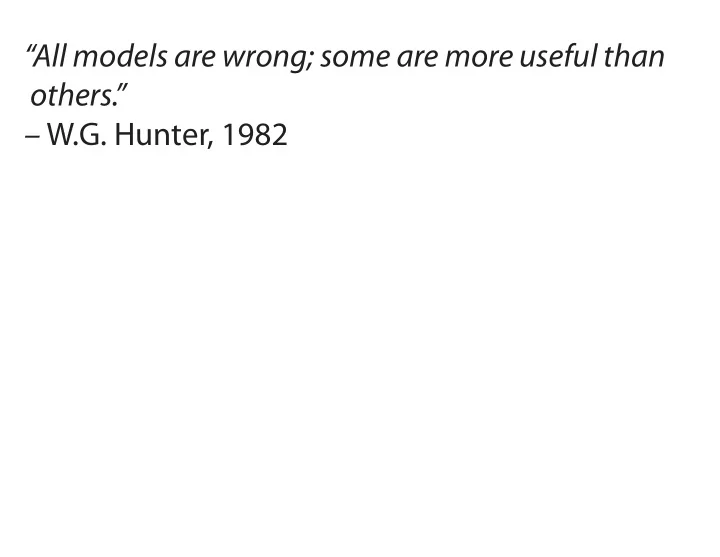
“All models are wrong; some are more useful than others.” – W.G. Hunter, 1982
“All models are wrong; some are more useful than others.” – W.G. Hunter, 1982 “Statisticians and artists have one thing in common. Neither should fall in love with their models.” – Gary Churchill, circa 1992
“If you think that thinking the earth is spherical is just as wrong as thinking the earth is flat, then your view is wronger than both of them put together.'' – Isaac Asimov. The relativity of wrong. The Skeptical Inquirer , 14(1):35–44, 1989.
Max. likelihood & Bayesian techniques are both likelihood-based. Weaknesses of likelihood for phylogeny reconstruction: 1) Computational tractability 2) Based on overly simplistic evolutionary models. But, a) All phylogeny reconstruction methods are based on assumptions but some (e.g. parsimony) are not based on explicit ones. For methods based on unstated assumptions, we need to worry not just whether the assumptions are realistic but also we need to worry about what they are. b) Likelihood methods allow assumptions to be rigorously tested. When an assumption is found to be particularly poor, it can be replaced with a better one (i.e., models will improve over time!)
Strengths of likelihood methods: 1. Explicit Assumptions – we know what we’re assuming. 2. Use all information in a data set. Distance methods, for example, do not. This is part of the explanation for success of likelihood methods in simulations – they tend to yield estimates that are closer to the truth than other methods. 3. Likelihood approaches are consistent. Estimates get better as amount of data increases. (Caveat: violation of model assumptions may cause loss of consistency property) 4. Because likelihood applied to so many statistical situations in addition to phylogenetics, powerful theory & tools for performing likelihood analyses have developed. This theory and these tools (e.g., tools for hypothesis testing) can be applied to phylogenetics. 5. Likelihood lets you know how good estimate is, in addition to what estimate is.
Mechanistic versus Phenomenological Models of Sequence Evolution see Ph.D. thesis by Nicolas Rodrigue (”Phylogenetic structural modeling of molecular evolution” , 2008, University of Montreal) (see also Rodrigue & Philippe. 2010. Trends in Genetics 26:248-252)
One good idea for more realistic models ... TUFFLEY, C., and M. A. STEEL. 1998. Modeling the covarion hypothesis of nucleotide substitution. Math. Biosci. 147:63–91.
From Galtier. 2001. Mol. Biol. Evol. 18(5):866-873.
Tuffley/Steel -type model Slow Fast A C G T A C G T A - r r r f 0 0 0 S C r - r r 0 f 0 0 l o G r r - r 0 0 f 0 w T r r r - 0 0 0 f A s 0 0 0 - q q q F C 0 s 0 0 q - q q a s G 0 0 s 0 q q - q t T 0 0 0 s q q q - Substitution Rates: q>r Switching rates: f (slow to fast), s (fast to slow)
Dayhoff model of protein evolution (see Dayhoff et al. 1972; Dayhoff et al. 1978) operates at the level of the 20 amino acid types. π is the probability of amino acid type i i α is the instantaneous rate of replacement from amino acid i ij to amino acid j Dayhoff model is most general time-reversible 20-state model of amino acid replacement. This means π α = π α for all i and j. i ij ji j
It is important to separate the Dayhoff model of protein evolution from: 1. The procedure used by Dayhoff and collaborators to estimate the α AND ij 2. The data set upon which the α estimates were based. ij Dayhoff and collaborators exploited the fact that the probability of replacements from amino acid type i to type j (i not equal to j) is approximately linear in time for small amounts of time. In other words, the probability of a replacement from amino acid type i to a different type j is approximately α t if t represents some ij small amount of time. Subsequent studies (e.g., Jones et al. 1992) adopted the Dayhoff model but employed different data sets and parameter estimation procedures.
Inspired by Lartillot and Philippe‛s CAT model of amino acid replacement that permits variation of preferred residues among sites, there is active development of sequence evolution models that allow variation of evolutionary processes among sites without prespecifying the number of categories, the nature of categories, or which sites are in which categories. Key Ingredient: “Dirichlet Process” as a prior for the number of categories and for the probabilities of the categories. Nicolas Lartillot and Hervé Philippe. 2004. A Bayesian Mixture Model for Across-Site Heterogeneities in the Amino-Acid Replacement Process. Mol. Biol. Evol. 21(6):1095-1109. 2004
Codon Models: Evolution occurs at the DNA level rather than at the amino acid level. It makes sense to frame a model of protein evolution in terms of codons rather than amino acid types (Schoniger et al. 1990; Goldman and Yang 1994; Muse and Gaut 1994). Codon-based models are typically framed in terms of 61 codon- states rather than 64 codon-states because the common genetic codes have three stop codons, and the possibility that a stop codon may appear or disappear from a sequence is not allowed. One simplification that is often adopted holds that changes from one codon to another are only possible when the two codons differ at exactly one of the three codon positions. The instantaneous rates of other changes between codons are set to 0.
Typical parameterization of a codon model when physicochemical differences between amino acids are ignored... Instantaneous rate α i,j from codon i to codon j is set to 0 if i and j differ at more than one nucleotide or if j encodes a premature stop codon. For cases where i and j differ by exactly one nucleotide, rate matrix entries are: for a synonymous transversion uπ j for a synonymous transition uπ j κ α i,j = for a nonsynonymous transversion uπ j ω uπ j κω for a nonsynonymous transition u , π j , and κ reflect mutation rates ω > 1 means positive diversifying selection (i.e., nonsyn. rates higher than they would be if changes were synonymous) Other kinds of positive selection exist (e.g., positive directional se- lection)
The previous rate matrix can be modified so that each codon k has its own parameter ω k . The rates then become: for a synonymous transversion uπ h for a synonymous transition uπ j κ α i,j = for a nonsynonymous transversion uπ j ω k uπ j κω k for a nonsynonymous transition As with the rate heterogeneity among sites treatment, the distribu- tion of ω k values among codons can be modelled. Often, we want to know if certain codons have ω k values that exceed 1.
Alternatively, we can assume all codons share the same value of ω but that ω values vary among branches on the tree. The rate matrix then becomes: for a synonymous transversion uπ j for a synonymous transition uπ j κ α i,j = for a nonsynonymous transversion uπ j ω B uπ j κω B for a nonsynonymous transition where ω B is the parameter value for branch B . Many other pos- sibilities for parameterizing codon models exist. and codon models can become very elaborate. For example, Pedersen and colleagues (1998) carefully designed a codon model to reflect the fact that CpG dinucleotide levels are depressed in lentiviral genes.
Codon models have received attention for their potential ability to detect positive selection (Nielsen and Yang 1998). Early methods for detecting positive selection from protein- coding DNA sequence data were designed to looked for an “excess” of nonsynonymous amino acid replacements throughout the sequence. Codon methods offer the potential of detecting positive selection at individual sites and for detecting the existence of a small proportion of sites at which positive selection may operate. Best statistical technique for detecting positive selection is a contentious issue at the moment...
Some future directions for codon-based models ... Evolutionary changes that simultaneously affect two consecutive positions could be allowed (Averof et al. 2000 have claimed empirical evidence for these kinds of changes). Reconciliation of codon-based models with classical population genetic models – some progress has been made (see Halpern and Bruno 1998). Improved treatment of effects of chemical similarity of amino acids on protein evolution
For change from Sequence i to Sequence j where i & j differ only at one sequence position, evolutionary rate from i to j is R where ij R = (Mutation Rate) x (Fixation Probability) ij (see Halpern & Bruno. 1998. MBE 15:910-917)
Recommend
More recommend
Explore More Topics
Stay informed with curated content and fresh updates.
