Algorithmic Paradigms Divide and Conquer Idea: Divide problem - PowerPoint PPT Presentation

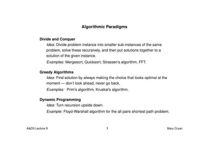
Algorithmic Paradigms Divide and Conquer Idea: Divide problem instance into smaller sub-instances of the same problem, solve these recursively, and then put solutions together to a solution of the given instance. Examples: Mergesort, Quicksort, Strassen’s algorithm, FFT. Greedy Algorithms Idea: Find solution by always making the choice that looks optimal at the moment — don’t look ahead, never go back. Examples: Prim’s algorithm, Kruskal’s algorithm. Dynamic Programming Idea: Turn recursion upside down. Example: Floyd-Warshall algorithm for the all pairs shortest path problem. 1 A&DS Lecture 9 Mary Cryan

Dynamic Programming - A Toy Example Fibonacci Numbers F 0 = 0, = F 1 1, = F n − 1 + F n − 2 F n (for n ≥ 2 ). A recursive algorithm Algorithm R EC -F IB ( n ) 1. if n = 0 then return 0 2. 3. else if n = 1 then return 1 4. 5. else return R EC -F IB ( n − 1 ) + R EC -F IB ( n − 2 ) 6. Ridiculously slow: exponentially many repeated computations of R EC -F IB ( j ) for small values of j . 2 A&DS Lecture 9 Mary Cryan

Fibonacci Example (cont’d) Why is the recursive solution so slow? Running time T ( n ) satisfies T ( n ) = T ( n − 1 ) + T ( n − 2 ) + Θ ( 1 ) ≥ F n ≈ 1.6 n . F n F F n−1 n−2 F F F F n−2 n−4 n−3 n−3 F F F F F F n−3 n−4 n−4 n−5 n−4 n−5 3 A&DS Lecture 9 Mary Cryan

Fibonacci Example (cont’d) Dynamic Programming Approach Algorithm D YN -F IB ( n ) 1. F [ 0 ] = 0 2. F [ 1 ] = 1 3. for i ← 2 to n do 4. F [ i ] ← F [ i − 1 ] + F [ i − 2 ] 5. return F [ n ] Running Time Θ ( n ) Very fast in practice - just need an array (of linear size) to store the F ( i ) values. 4 A&DS Lecture 9 Mary Cryan

Multiplying Sequences of Matrices Recall Multiplying a ( p × q ) matrix with a ( q × r ) matrix (in the standard way) requires pqr multiplications. We want to compute products of the form A 1 · A 2 · · · A n . How do we set the parentheses? 5 A&DS Lecture 9 Mary Cryan

Example Compute A B C D · · · 30 × 1 1 × 40 40 × 10 10 × 25 Multiplication order ( A · B ) · ( C · D ) requires 30 · 1 · 40 + 40 · 10 · 25 + 30 · 40 · 25 = 41, 200 multiplications. Multiplication order A · (( B · C ) · D ) requires 1 · 40 · 10 + 1 · 10 · 25 + 30 · 1 · 25 = 1, 400 multiplications. 6 A&DS Lecture 9 Mary Cryan

The Matrix Chain Multiplication Problem Input: Sequence of matrices A 1 , . . . , A n , where A i is a p i − 1 × p i -matrix Output: Optimal number of multiplications needed to compute A 1 · A 2 · · · A n and optimal parenthesisation Running time of algorithms will be measured in terms of n . 7 A&DS Lecture 9 Mary Cryan

Solution Attempts Approach 1: Exhaustive search. Try all possible parenthesisations and compare them. Correct, but extremely slow; running time is Ω ( 3 n ) . Approach 2: Greedy algorithm. Always do the cheapest multiplication first. Does not work correctly — sometimes, it returns a parenthesisation that is not optimal: Example: Consider A 1 A 2 A 3 · · 3 × 100 100 × 2 2 × 2 Solution proposed by greedy algorithm: A 1 · ( A 2 · A 3 ) with 100 · 2 · 2 + 3 · 100 · 2 = 1000 multiplications. Optimal solution: ( A 1 · A 2 ) · A 3 with 3 · 100 · 2 + 3 · 2 · 2 = 612 multiplications. 8 A&DS Lecture 9 Mary Cryan

Solution Attempts (cont’d) Approach 3: Alternative greedy algorithm. Set outermost parentheses such that cheapest multiplication is done last. Doesn’t work correctly either (Exercise!). Approach 4: Recursive (Divide and Conquer). Divide: ( A 1 · · · A k ) · ( A k + 1 · · · A n ) For all k , recursively solve the two sub-problems and then take best overall solution. For 1 ≤ i ≤ j ≤ n , let m [ i, j ] = least number of multiplications needed to compute A i · · · A j Then � if i = j, 0 m [ i, j ] = ` ´ m [ i, k ] + m [ k + 1, j ] + p i − 1 p k p j if i < j. min 1 ≤ k<j 9 A&DS Lecture 9 Mary Cryan

Analysis of the Recursive Algorithm Running time T ( n ) satisfies the recurrence n − 1 � � � T ( n ) = T ( k ) + T ( n − k ) + Θ ( n ) . k = 1 This implies T ( n ) = Ω ( 2 n ) . 10 A&DS Lecture 9 Mary Cryan

Dynamic Programming Solution As before: m [ i, j ] = least number of multiplications needed to compute A i · · · A j Moreover, s [ i, j ] = (the smallest) k such that i ≤ k < j and m [ i, j ] = m [ i, k ] + m [ k + 1, j ] + p i − 1 p k p j . s [ i, j ] can be used to reconstruct the optimal parenthesisation. Idea Compute the m [ i, j ] and s [ i, j ] in a bottom-up fashion. 11 A&DS Lecture 9 Mary Cryan

Implementation Algorithm M ATRIX -C HAIN -O RDER ( p ) 1. n ← p. length − 1 2. for i ← 1 to n do 3. m [ i, i ] ← 0 4. for ℓ ← 2 to n do for i ← 1 to n − ℓ + 1 do 5. 6. j ← i + ℓ − 1 7. m [ i, j ] ← ∞ for k ← i to j − 1 do 8. 9. q ← m [ i, k ] + m [ k + 1, j ] + p i − 1 p k p j if q < m [ i, j ] then 10. 11. m [ i, j ] ← q 12. s [ i, j ] ← k 13. return s Running Time: Θ ( n 3 )

Example A 1 A 2 A 3 A 4 · · · 30 × 1 1 × 40 40 × 10 10 × 25 Solution for m and s m 1 2 3 4 s 1 2 3 4 1 0 1200 700 1400 1 1 1 1 2 0 400 650 2 2 3 3 0 10 000 3 3 4 0 4 Optimal Parenthesisation A 1 · (( A 2 · A 3 ) · A 4 )) 13 A&DS Lecture 9 Mary Cryan

Multiplying the Matrices Algorithm M ATRIX -C HAIN -M ULTIPLY ( A, p ) 1. n ← A. length 2. s ← M ATRIX -C HAIN -O RDER ( p ) 3. return R EC -M ULT ( A, s, 1, n ) Algorithm R EC -M ULT ( A, s, i, j ) 1. if i < j then 2. C ← R EC -M ULT ( A, s, i, s [ i, j ]) 3. D ← R EC -M ULT ( A, s, s [ i, j ] + 1, j ) return ( C ) · ( D ) 4. 5. else return A i 6. 14 A&DS Lecture 9 Mary Cryan

Reading Assignment see Wikipedia: http://en.wikipedia.org/wiki/Dynamic programming [CLRS] Sections 15.2-15.4 (pages 331-356) This is Sections 16.1-16.3 (pages 302-320) of [CLR]. Problems 1. Review the Edit-Distance Algorithm (Inf2B cwk 3 in 06/07) and try to understand why it is a dynamic programming algorithm. 2. Exercise 15.2-1, p.338 of [CLRS] or 16.1-1, p.308 of [CLR]. 15 A&DS Lecture 9 Mary Cryan