Algorithm-based checkpoint-recovery for the conjugate gradient - PowerPoint PPT Presentation
Algorithm-based checkpoint-recovery for the conjugate gradient method Carlos Pachajoa, Christina Pacher, Markus Levonyak, Wilfried N. Gansterer. 49th International Conference on Parallel Processing Acknowledgements This work has been funded by
Algorithm-based checkpoint-recovery for the conjugate gradient method Carlos Pachajoa, Christina Pacher, Markus Levonyak, Wilfried N. Gansterer. 49th International Conference on Parallel Processing
Acknowledgements This work has been funded by the Vienna Science and Technology Fund through project ICT15-113. Experiments are run on the VSC3 machine of the Vienna Scientific Cluster.
Motivation 1 Unreliability at larger scales • Reliability of larger-scale computer systems is predicted to decline. • Computers can no longer be thought as reliable machines. Resilience is an active research field. • We focus on node failures: Events in which a node stops working and the data contained in it is lost. Several nodes can fail simultaneously if, for example, a switch stops working. 2 Resilience for the conjugate gradient method • Iterative solver for symmetric, positive definite (SPD) linear systems. • Significant in many physically-motivated problems. • Particularly suitable for work with sparse matrices. Usable in very large systems.
Problem statement • Unreliable computer cluster. Possibility of node failures occuring. • Find the solution of a linear system for an SPD matrix using the conjugate gradient method. • Sparse matrices stored with a block-row distribution. Vector elements distributed in the same way as the rows.
Key idea 1: Matrix-vector product • The matrix-vector product provides some redundancy for the input vector, and can be augmented to guarantee complete redundancy.
Storing redundantly for a node failure The matrix-vector product provides some redundancy for the input vector (Chen 2011). In this example, we focus on the second rank: One of its entries is not necessary for the SpMV and must be sent additionally. Node 0 Node 1 Ap = Node 2 Node 3
Multiple node failures • These ideas can be generalized to deal with multiple, simultaneous node failures, for example, in the event of a switch failure.
Augmented SpMV product for multiple node failures m i : Multiplicity of entry i . m 4 = 2 m 5 = 0 m 6 = 2 m 7 = 1 Node 0 Node 1 Ap = Node 2 Node 3 To guarantee we can recover from up to φ node failures, the SpMV must be augmented until the multiplicity for every entry of each node is m i ≥ φ
Key idea 2: State reconstruction The complete state can be recovered from the two last search directions (the p vector) (Pachajoa et al. 2019). Exact state reconstruction method Preconditioned conjugate gradient method Retrieve the static data A If , I , P If , I , and b If ; 1 Gather r ( j ) I \ If and x ( j ) I \ If ; 2 r (0) := b − Ax (0) , z (0) := Pr (0) , p (0) := z (0) 1 Retrieve the redundant copies of β ( j − 1) , p ( j − 1) , and p ( j ) If ; repeat 3 2 If α ( j ) := r ( j ) ⊤ z ( j ) / p ( j ) ⊤ Ap ( j ) ; Compute z ( j ) := p ( j ) − β ( j − 1) p ( j − 1) 3 ; 4 x ( j +1) := x ( j ) + α ( j ) p ( j ) ; If If If 4 Compute v := z ( j ) − P If , I \ If r ( j ) I \ If ; r ( j +1) := r ( j ) − α ( j ) Ap ( j ) ; 5 If 5 z ( j +1) := Pr ( j +1) ; Solve P If , If r ( j ) = v for r ( j ) If ; 6 6 If β ( j ) := r ( j +1) ⊤ z ( j +1) / r ( j ) ⊤ z ( j ) ; 7 Compute w := b If − r ( j ) − A If , I \ If x ( j ) I \ If ; 7 p ( j +1) := z ( j +1) + β ( j ) p ( j ) ; If 8 Solve A If , If x ( j ) = w for x ( j ) If ; until � r � 2 / � b � 2 < rtol ; 9 8 If
Key idea 3: Reduce the overhead by storing every T iterations ESR algorithm Retrieve the static data A If , I , P If , I , and b If ; 1 2 3 4 5 6 1 + + + + + + Gather r ( j ) I \ If and x ( j ) I \ If ; 2 j j j j j j j Retrieve the redundant copies of β ( j − 1) , p ( j − 1) , and p ( j ) If ; 3 If Compute z ( j ) := p ( j ) − β ( j − 1) p ( j − 1) ; 4 If If If p ( j ) p ( j +1) p ( j +2) p ( j +3) p ( j +4) p ( j +5) p ( j +6) Compute v := z ( j ) − P If , I \ If r ( j ) I \ If ; 5 If x ( j ) x ( j +1) x ( j +2) x ( j +3) x ( j +4) x ( j +5) x ( j +6) Solve P If , If r ( j ) = v for r ( j ) If ; 6 If z ( j ) z ( j +1) z ( j +2) z ( j +3) z ( j +4) z ( j +5) z ( j +6) Compute w := b If − r ( j ) − A If , I \ If x ( j ) I \ If ; 7 r ( j ) r ( j +1) r ( j +2) r ( j +3) r ( j +4) r ( j +5) r ( j +6) If Solve A If , If x ( j ) = w for x ( j ) If ; 8 If Two problems: • To use the reconstructed parts, we also need the corresponding entries of the vector for that iteration. • Therefore, all nodes must store their local parts of the vector at the checkpoint. • We need p for two consecutive iterations to be able to perform the reconstruction. • We need a queue of redundantly stored data.
Storing redundant data every few iterations 1 1 2 1 1 2 − + + − + + T T T T T T T T 0 1 2 2 2 2 = = = = = = = = = = j j j j j j j j j j Start ] ] ] ] ] ] ] ] ] ] ) ) ) ) ) ) ) 1 1 1 1 1 T T , , , + + + + + ( 2 , , , ′ ( T T T T T p ′ [ [ [ ( ( ( 2 2 p ′ ′ ′ ( ( , p p p ′ ′ , ) p p , 1 , , , ) ) ) + , , [ ) ) T T T T T T ( ( ( ′ ′ ′ ( 2 2 p p p ′ ( ( p ′ ′ , , , p p , ) [ [ [ , , ) ) T 1 1 ( + + ′ p T T [ ( ( ′ ′ p p [ [
Definition of ASpMV • The function SpMV takes a matrix and a vector as inputs, and outputs a ̺ := SpMV ( A , p ) vector. • The function ASpMV additionally takes ̺ := ASpMV ( A , p , φ, Q ) a target number of redundant copies ( φ ) and a queue to store them ( Q ).
Reducing the frequency: CG-ESRP Conjugate gradient method using exact state reconstruction with periodic storage (CG-ESRP) 1 r (0) := b − Ax (0) , z (0) := Pr (0) , p (0) := z (0) , j := 0 , 2 Q := [ , , ]; Preconditioned conjugate gradient method 3 repeat if j mod T = 0 and j > 2 then 4 ̺ ( j ) := ASpMV ( A , p ( j ) , φ, Q ); 1 r (0) := b − Ax (0) , z (0) := Pr (0) , p (0) := z (0) 5 β ∗ ∗ = β ( j ) ; 6 2 repeat ( j − 1) mod T = 0 and j > 2 then else if 7 α ( j ) := r ( j ) ⊤ z () / p ( j ) ⊤ Ap ( j ) ; ̺ ( j ) := ASpMV ( A , p ( j ) , φ, Q ); 3 8 x ( j +1) := x ( j ) + α ( j ) p ( j ) ; x ∗ = x ( j ) , r ∗ = r ( j ) , z ∗ = z ( j ) , p ∗ = p ( j ) ; 4 9 β ∗ = β ∗ ∗ ; 10 r ( j +1) := r ( j ) − α ( j ) Ap ( j ) ; 5 else 11 z ( j +1) := Pr ( j +1) ; ̺ ( j ) := SpMV ( A , p ( j ) ); 6 12 α ( j ) := r ( j ) ⊤ z ( j ) / p ( j ) ⊤ ̺ ( j ) ; β ( j ) := r ( j +1) ⊤ z ( j +1) / r ( j ) ⊤ z ( j ) ; 13 7 x ( j +1) := x ( j ) + α ( j ) p ( j ) ; 14 p ( j +1) := z ( j +1) + β ( j ) p ( j ) ; 8 r ( j +1) := r ( j ) − α ( j ) ̺ ( j ) ; 15 9 until � r � 2 / � b � 2 < rtol ; z ( j +1) := Pr ( j +1) ; 16 β ( j ) := r ( j +1) ⊤ z ( j +1) / r ( j ) ⊤ z ( j ) ; 17 p ( j +1) := z ( j +1) + β ( j ) p ( j ) ; 18 j := j + 1; 19 20 until � r � 2 / � b � 2 < rtol ;
Experimental setup • 128 nodes of the VSC3. • Two strategies to recover: ESRP and in-memory CR (IMCR). • Simulated node failures. • Checkpointing interval of 20, 50 and 100 iterations. • Resilience with 1, 3 and 8 redundant copies. • Runs without resilience, and with resilience with and without node failures. Test matrices from the SuiteSparse collection (Davis and Hu 2011) Matrix Problem type Problem size #NZ Emilia 923 Structural 923 136 40 373 538 audikw 1 Structural 943 695 77 651 847
Results for matrix Emilia 923 • Reference time t 0 = 14 . 66 s • σ t 0 is 0.93% of t 0 . 10.0% ESRP 10.0% ESR IMCR runtime overhead runtime overhead 1.0% ESRP ESR 0.1% IMCR 1.0% T = 20 T = 50 T = 100 T = 20 T = 50 T = 100 checkpointing interval checkpointing interval (a) Failure-free solver (b) Node failures introduced
Results for matrix audikw 1 • Reference time t 0 = 23 . 22 s • σ t 0 is 0.14% of t 0 . 10.0% runtime overhead runtime overhead 1.0% ESRP ESRP 1.0% 0.1% ESR ESR IMCR IMCR T = 20 T = 50 T = 100 T = 20 T = 50 T = 100 checkpointing interval checkpointing interval (a) Failure-free solver (b) Node failures introduced
Conclusions and perspectives Conclusions • In our first experiments, ESRP drastically reduces the overhead of ESR. • In failure-free cases, also faster than in-memory CR. • In our experiments, the cost of communication seems to be too low. We cannot conclude that IMCR is faster than ESRP in this case. • Recovery time for ESRP is dominated by the solution of the local linear system during reconstruction. Perspectives • Experiments with larger problems and a larger number of nodes, to reach a different regime for computation/communication ratio. • Application of matrix partitioning algorithms. • Implementation with real node failures.
Contact us REPEAL Project https://repeal.taa.univie.ac.at/ Carlos Pachajoa carlos.pachajoa@univie.ac.at
Recommend
More recommend
Explore More Topics
Stay informed with curated content and fresh updates.

