Algebraic Voting Theory Michael Orrison Harvey Mudd College - PowerPoint PPT Presentation
Algebraic Voting Theory Michael Orrison Harvey Mudd College Collaborators and Sounding Boards Don Saari (UC Irvine) Anna Bargagliotti (University of Memphis) Steven Brams (NYU) Brian Lawson (Santa Monica College) Zajj Daugherty 05 Alex
Algebraic Voting Theory Michael Orrison Harvey Mudd College
Collaborators and Sounding Boards Don Saari (UC Irvine) Anna Bargagliotti (University of Memphis) Steven Brams (NYU) Brian Lawson (Santa Monica College) Zajj Daugherty ’05 Alex Eustis ’06 Mike Hansen ’07 Marie Jameson ’07 Gregory Minton ’08 Stephen Lee ’10 Jen Townsend ’10 (Scripps) Aaron Meyers ’10 (Bucknell) Sarah Wolff ’10 (Colorado College) Angela Wu ’10 (Swarthmore)
Voting Paradoxes
Voting–Preferences Example Eleven voters have the following preferences: 2 ABC 3 ACB 4 BCA 2 CBA. We will call this voting data the profile. Change of Perspective Focus on the procedure, not the preferences, because “...rather than reflecting the views of the voters, it is entirely possible for an election outcome to more accurately reflect the choice of an election procedure.” (Donald Saari, Chaotic Elections! )
Let’s Vote! Preferences 2 ABC 3 ACB 4 BCA 2 CBA Plurality: Vote for Favorite A: 5 points B: 4 points C: 2 points A > B > C Anti-Plurality: Vote for Top Two Favorites A: 5 points B: 8 points C: 9 points C > B > A Borda Count: 1 Point for First, 1 2 Point for Second C: 5 1 A: 5 points B: 6 points 2 points B > C > A
Algebraic Perspective
Positional Voting with Three Candidates Weighting Vector: w = [1 , s , 0] t ∈ R 3 1st: 1 point 2nd: s points, 0 ≤ s ≤ 1 3rd: 0 points Tally Matrix: T w : R 3! → R 3 2 ABC 3 ACB 1 1 s 0 s 0 5 A 0 BAC T w ( p ) = s 0 1 1 0 s = 4 + 4 s B = r 4 BCA 0 0 1 1 2 + 7 s C s s 0 CAB 2 CBA
Linear Algebra Tally Matrices In general, we have a weighting vector w = [ w 1 , . . . , w n ] t ∈ R n and T w : R n ! → R n . Profile Space Decomposition The effective space of T w is E ( w ) = (ker( T w )) ⊥ . Note that R n ! = E ( w ) ⊕ ker( T w ) . Questions What is the dimension of E ( w )? Given w and x , what is E ( w ) ∩ E ( x )?
Change of Perspective Profiles We can think of our profile 2 ABC 3 ACB 0 BAC p = 4 BCA 0 CAB 2 CBA as an element of the group ring R S 3 : p = 2 e + 3(23) + 0(12) + 4(123) + 0(132) + 2(13) .
Change of Perspective Tally Matrices We can think of our tally T w ( p ) as the result of p acting on w : 2 3 1 1 0 0 1 1 0 0 s s 0 + 3 + 4 + 2 T w ( p ) = 0 1 1 0 = 2 0 1 s s s s 4 0 0 1 1 0 1 s s s s 0 2 1 = p · w . = (2 e + 3(23) + 4(123) + 2(13)) · s 0
Representation Theory We have elements of R S n (i.e., profiles) acting as linear transformations on the vector space R n : ρ : R S n → End( R n ) ∼ = R n × n . This opens the door to using tools and insights from the representation theory of the symmetric group.
Theorems
Equivalent Weighting Vectors Defintion Two nonzero weighting vectors w , x ∈ R n are equivalent ( w ∼ x ) if and only if there exist α, β ∈ R such that α > 0 and x = α w + β 1 . Example [3 , 2 , 1] t ∼ [2 , 1 , 0] t ∼ [1 , 1 / 2 , 0] t ∼ [1 , 0 , − 1] t Sum-zero Weighting Vectors For convenience, we will usually assume that the entries of our weighting vectors sum to zero, i.e., our weighting vectors are sum-zero vectors. Key Insight If w � = 0 is sum-zero, then E ( w ) is an irreducible R S n -module. In fact, E ( w ) ∼ = S ( n − 1 , 1) .
Results Theorem (Saari) Let n ≥ 2 , and let w and x be nonzero weighting vectors in R n . The ordinal rankings of T w ( p ) and T x ( p ) will be the same for all p ∈ R n ! if and only if w ∼ x . Theorem If w and x are nonzero sum-zero weighting vectors in R n , then E ( w ) = E ( x ) if and only if w ∼ x . Moreover, if E ( w ) � = E ( x ) , then E ( w ) ∩ E ( x ) = { 0 } . Theorem If w and x are nonzero sum-zero weighting vectors in R n , then w ⊥ x if and only if E ( w ) ⊥ E ( x ) .
Results Theorem Let n ≥ 2 , and suppose { w 1 , . . . , w k } ⊂ R n is a linearly independent set of sum-zero weighting vectors. If r 1 , . . . , r k are any k sum-zero results vectors in R n , then there exist infinitely many profiles p ∈ R n ! such that T w i ( p ) = r i for all 1 ≤ i ≤ k. In other words... For a fixed profile p , as long as our weighting vectors are different enough, there need not be any relationship whatsoever among the results of each election. Key to the Proof A theorem by Burnside says that every linear transformation from an irreducible module to itself can be realized as the action of some element (i.e., a profile) in R S n .
Why the Borda Count is Special
Pairwise Voting Ordered Pairs Assign points to each ordered pair of candidates, then use this information to determine a winner. Example of the Pairs Matrix 1 1 0 0 1 0 2 ABC 5 AB 0 0 1 1 0 1 3 ACB 6 BA 1 1 1 0 0 0 0 BAC 5 AC P 2 ( p ) = = 0 0 0 1 1 1 4 BCA 6 CA 1 0 1 1 0 0 0 CAB 6 BC 0 1 0 0 1 1 2 CBA 5 CB Voting Connection Some voting procedures (e.g., Copeland) depend only on P 2 ( p ).
Pairwise and Positional Voting Question How are pairwise and positional voting methods related? Definition Let T and T ′ be linear transformations defined on the same vector space V . We say that T is recoverable from T ′ if there exists a linear transformation R such that T = R ◦ T ′ . Theorem (Saari) A tally map T w : R n ! → R n is recoverable from the pairs map P 2 : R n ! → R n ( n − 1) if and only if w is equivalent to the Borda count [ n − 1 , n − 2 , . . . , 1 , 0] . Key to Our Proof = S ( n − 1 , 1) and E ( P 2 ) ∼ = S ( n ) ⊕ S ( n − 1 , 1) ⊕ S ( n − 2 , 1 , 1) . E ( T w ) ∼
Counting Questions To find the number of times each candidate is ranked above a ( k − 1)-element subset of other candidates, use the weighting vector �� n − 1 � � n − 2 � � � � �� 1 0 b k = , , . . . , , . k − 1 k − 1 k − 1 k − 1 This is a generalization of the Borda count (which is b 2 ). Example If n = 4, then b 1 = [1 , 1 , 1 , 1], b 2 = [3 , 2 , 1 , 0], b 3 = [3 , 1 , 0 , 0], and b 4 = [1 , 0 , 0 , 0].
Generalized Specialness k -wise Maps Generalize the pairwise map P 2 to create the k-wise map P k : R n ! → R ( n ) k where P k counts the number of times each ordered k -tuple of candidates is actually ranked in that order by a voter. Theorem Let n ≥ 2 and let w ∈ R n be a weighting vector. The map T w is recoverable from the k-wise map P k if and only if w is a linear combination of b 1 , . . . , b k . Definition We say that a weighting vector is k -Borda if it is a linear combination of b 1 , . . . , b k .
Orthogonal Bases Applying Gram-Schmidt to the b i for small values of n yields: n = 2: c 1 = [1 , 1], c 2 = [1 , − 1] n = 3: c 1 = [1 , 1 , 1], c 2 = [2 , 0 , − 2], and c 3 = [1 , − 2 , 1]. n = 4: c 1 = [1 , 1 , 1 , 1], c 2 = [3 , 1 , − 1 , − 3], c 3 = [3 , − 3 , − 3 , 3], and c 4 = [1 , − 3 , 3 , − 1]. Theorem A weighting vector for n candidates is ( n − 1) -Borda if and only if it is orthogonal to the nth row of Pascal’s triangle with alternating signs. Proof. Focus on the inverses of so-called Pascal matrices.
Pascal Matrices If n = 5, then we are interested in the following Pascal matrix: 1 0 0 0 0 1 1 0 0 0 1 2 1 0 0 . 1 3 3 1 0 1 4 6 4 1 Its inverse looks just like itself but with alternating signs: 1 0 0 0 0 − 1 1 0 0 0 1 − 2 1 0 0 . − 1 3 − 3 1 0 1 − 4 6 − 4 1
Tests of Uniformity
Profiles Ask m people to fully rank n alternatives from most preferred to least preferred, and encode the resulting data as a profile p ∈ R n ! . Example If n = 3, and the rankings of the alternatives A , B , C are ordered lexicographically, then the profile p = [10 , 15 , 2 , 7 , 9 , 21] t ∈ R 6 encodes the situation where 10 judges chose the ranking ABC , 15 chose ACB , 2 chose BAC , and so on.
Data from a Distribution We imagine that the data is being generated using a probability distribution P defined on the permutations of the alternatives. We want to test the null hypothesis H 0 that P is the uniform distribution. A natural starting point is the estimated probabilities vector � P = (1 / m ) p . If � P is far from the vector (1 / n !)[1 , . . . , 1] t , then we would reject H 0 . In general, given a subspace S that is orthogonal to [1 , . . . , 1] t , we’ll compute the projection of � P onto S , and we’ll use the value mn ! � � P S � 2 as a test statistic.
Recommend
More recommend
Explore More Topics
Stay informed with curated content and fresh updates.


