Aix-en-Provence (France) 7-9 November 2005 Session II: Methods for - PowerPoint PPT Presentation

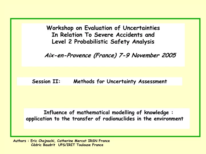
Workshop on Evaluation of Uncertainties In Relation To Severe Accidents and Level 2 Probabilistic Safety Analysis Aix-en-Provence (France) 7-9 November 2005 Session II: Methods for Uncertainty Assessment Influence of mathematical modelling of knowledge : application to the transfer of radionuclides in the environment Authors : Eric Chojnacki, Catherine Mercat IRSN France Cédric Baudrit UPS/IRIT Toulouse France

Influence of mathematical modelling of knowledge : application to the transfer of radionuclides in the environment Contents 1°) Introduction : limits of MC-methods 2°) Fuzzy modelling : an extension of interval calculation 3°) Links between fuzzy numbers and possibility theory 4°) Dempster-Shafer theory : an unified framework 5°)‘Dempster-Shafer’ uncertainty methodology 6°) Application to a simple example 7°) Conclusion

Introduction : limits of MC-methods Monte-Carlo methods need a lot of knowledge. 1 ° ) Choice of the input PDFs Example of uniform distribution Ignorance does not mean equiprobability 2 ° ) Knowledge of possible dependencies between uncertain parameters Example of independence assumption No dependence information does not mean stochastic independence . Such assumptions may lead to an artificial reduction of uncertainty margins and thus can deteriorate the relevance of the decision making.

Current practices to mitigate difficulties encountered in MC simulations • Use of deterministic penalizing values • Use of penalizing PDFs or penalizing dependencies • Double MC techniques • Use of fuzzy theory • Hybrid theory : a combination of fuzzy and probability theories

Fuzzy modelling : an extension of interval calculation Definition 1 : a fuzzy set is an extension of a classical set, with a membership function instead of a characteristic function Definition 2 : an α -cut is the set of points with a membership ≥ α . Definition 3 : a fuzzy number is a fuzzy set for which the α -cuts are nested intervals I α : I 1 ⊂ I α I 0 ⊂ Example 1 : a flat fuzzy number A membership function 1 I α I α = [ A min , A max ] ∀α ∈ [0 , 1] 0 A min A max Example 2 : a triangular fuzzy number A membership function 1 I α I α = [ A min + α (A nom - A min ) , A max - α (A max - A nom ) ] 0 A max A min A nom

Fuzzy modelling : an extension of interval calculation Trapezoidal fuzzy number A = (1, 2, 4, 7). Triangular fuzzy number B = (2, 3, 4). 1,2 1,2 1 1 ip ip I 0.6 0,8 0,8 h h rs rs I 0.6 e e 0,6 A 0,6 B b b m m e 0,4 e 0,4 m m 0,2 0,2 0 0 0 2 4 6 8 1 2 3 4 5 Interval A = [ 1 , 7 ] Interval B = [ 2 , 4 ] Results : A+B, A*B, A/B 1,2 1 0,8 A+B 0,6 A*B A/B 0,4 0,2 0 0 10 20 30 A*B = [ 2 , 28 ] A/B = [ 0.25 , 3.5 ] A+B = [ 3 , 11 ] The fuzzy calculation is an interval calculation performed for each α -cut I α

Links between possibility theory and probability theory A possibility measure as a probability measure is a way to measure the confidence associated to an event. By definition, a possibility measure must satisfy the three following axioms : π ( ∅ )=0, π (E)= 1 where E is the whole set, π (A ∪ B)=max( π (A), π (B)) for any subsets A and B. Let us remind the Kolmogorov axioms of a probability measure P : P( ∅ )=0, P(E)= 1 where E is the whole set, P(A ∪ B)= P(A) + P(B) for any subsets A and B such as A ∩ B= ∅ . N.B 1 π (A)=1 and π (non A)= 1 means that no information on the occurrence of the event A is known. N.B 2 π (A)=0 means that the event A is impossible, therefore π (non A)= 1 .

Links between fuzzy numbers and possibility theory Example : Quantity of ingested fish Q 1 fish μ (30)=0.5 μ (40)=1.0 μ (50)=0.75 μ membership μ (60)=0.5 μ (70)=0.25 μ (80)=0. 0 20 30 40 50 60 70 80 A membership function measures the membership of an element to a fuzzy set. A membership function does not allow to measure the confidence associated to an event. A membership function allows to define a possibility measure from which it is possible to measure the confidence associated to an event.

Links between fuzzy numbers and possibility theory Example : Quantity of ingested fish Q Possibility π 1 fish π ({40}) = 1.0 π ([20,30] )= 0.5 π ([70,80] )= 0.25 π ([70,80] ∪ [20,30])=0.5 0 20 30 40 50 60 70 80 A fuzzy number defines a possibility distribution: π (E)= π (E knowing Q)= max ( μ (x)) x ∈ E

Links between possibility theory and probability theory A possibility distribution is similar to a family of PDFs Example : triangular possibility Equivalent set of PDFs possibility distribution ingested fish ingested fish 1 1 triangular law 0 0 20 30 40 50 60 70 80 20 30 40 50 60 70 80 imprecision A triangular distribution of possibility contents all the probabilities with the same mode and support.

Dempster-Shafer theory: an unified framework for possibility and probability theories Possibility Probability 0.2 0.2 A 1 A 2 A 3 A 4 A 5 0.2 A 5 A 4 0.2 A 3 A 2 A 1 0.2 0.05 0.15 0.3 0.3 0.2 A 3 m(A 1 )=0.2 m(A 2 )=0.4 A 2 A 1 m(A 3 )=0.2 A 1 m(A 4 )=0.2 A 4 Dempster-Shafer

Dempster-Shafer theory: an unified framework for possibility and probability theories Uncertainty propagation : the ‘Dempster-Shafer’ method Principle = extended MC simulations Model = M(X 1 ,…,X k ,X k+1 ,…,X n ); X 1 ,…,X k probabilities and X k+1 ,…,X n possibilities Variable X k If variability: enough knowledge Variable X 1 1 1 available p 1 . . . p k PDF 0 0 x 1 x k X n If imprecision: not enough Variable Variable X k+1 1 1 knowledge available α k +1 α n . . . family of PDFs 0 0 encoded by α α -cut of X k+1 -cut of X n a possibility distribution Result = sample of random intervals

Dempster-Shafer theory: an unified framework for possibility and probability theories How to evaluate the uncertainty of an event? For example x Є [3,7] Example of results: 1 5 ν 1 lower probability upper probability 2 6 ν 2 ν 3 ≤ Proba(x Є [3, 7]) ≤ ν 1 + ν 2 + ν 3 + ν 4 3.5 6.5 ν 3 3 7 0 4 ν 4 In MC simulations all the ν i = 1/N

Application to a simple example A simple radionuclide transfer model from maize to man through the consumption of milk Absorbed dose D = A * Q* F * M A : the maize activity is a random variable, known from experimental measurement Q : the quantity of eaten maize : very likely between 10 and 14 kg/day and cannot be out of the interval [4 , 35], F : the transfer factor from maize to milk in the interval [0.001 , 0.005] with 0.003 day/litre for the most likely value, M : the quantity of ingested milk in the interval [70 , 280] with 140 litre/year for the most likely value. The knowledge related to the parameters Q, F, M is not enough to define a specific PDF. The set of PDFs checking these conditions can be easily encoded by the mean of possibility distributions.

Application to a simple example Modelling of dependencies between uncertainty ‘sources’ Stochastic independency and epistemic independency Stochastic independency. The stochastic independency between two uncertain variables means that there is slight likely to have simultaneously extreme values between random variables and leads to a compensating effect between uncertainty sources. Epistemic independency The epistemic independency assumes that the information related to the two uncertain variables have the same reliability. With this assumption, the uncertainties may cumulate themselves . Property : Epistemic independency is similar to an ignorance of the stochastic dependency. Indeed, the use of the epistemic independency as in the interval calculation, leads to cumulate uncertainties when no information is available about compensating effects. At the opposite, the use of stochastic independence assumptions, when it is possible, limits the over-conservatism of standard interval calculations.

Application to a simple example Modelling of uncertainty ‘sources’ parameter Probabilistic methods : Dempster-Shafer methods P_SI and P_EI DS_SI and DS_EI maize random variable : random variable : activity lognormal distribution lognormal distribution m=-5.76 , σ =0.58 m=-5.76 , σ =0.58 A quantity of random variable : fuzzy variable : maize trapezoidal distribution trapezoidal distribution Q (4, 10, 14, 35) (4, 10, 14, 35) transfer random variable : fuzzy variable : factor triangular distribution triangular distribution F (0.001, 0.003, 0.005) (0.001, 0.003, 0.005) quantity of random variable : fuzzy variable : milk triangular distribution triangular distribution M (70, 140, 280) (70, 140, 280) _SI for Stochastic Independence assumption and _EI for Epistemic Independence assumption

Application to a simple example Result : CCDF of the activity Dose 1 0,9 P_SI 0,8 l e 0,7 P_EI v le 0,6 DS_EI e percentile 95% c 0,5 n DS_SI e 0,4 fid DS_EI 0,3 n o 0,2 c DS_SI 0,1 0 0 0,1 0,2 0,3 0,4 0,5 Bq/year

Application to a simple example PDF effect with Epistemic Independence 0.16 0.34 0.01 0.03 PDF effect with Stochastic Independence Percentile 95% derived from MC simulations Conclusion : These figure shows the importance of the assumptions related to the choice of marginal distributions (a factor ~10 on the percentile 95% ) and their dependencies (a factor ~3 on the percentile 95% ) on the uncertainty margins.