Aix-en-Provence (France) 7-9 November 2005 Session II: Methods for - PowerPoint PPT Presentation
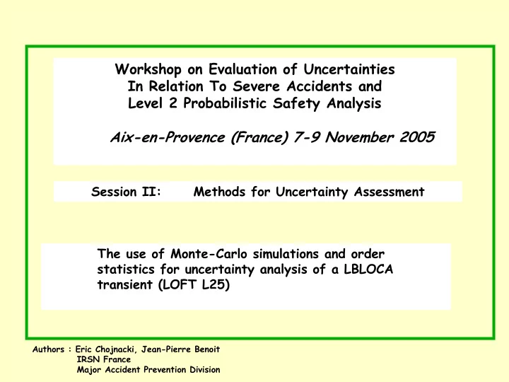
Workshop on Evaluation of Uncertainties In Relation To Severe Accidents and Level 2 Probabilistic Safety Analysis Aix-en-Provence (France) 7-9 November 2005 Session II: Methods for Uncertainty Assessment The use of Monte-Carlo simulations and
Workshop on Evaluation of Uncertainties In Relation To Severe Accidents and Level 2 Probabilistic Safety Analysis Aix-en-Provence (France) 7-9 November 2005 Session II: Methods for Uncertainty Assessment The use of Monte-Carlo simulations and order statistics for uncertainty analysis of a LBLOCA transient (LOFT L25) Authors : Eric Chojnacki, Jean-Pierre Benoit IRSN France Major Accident Prevention Division
Workshop on Evaluation of Uncertainties In Relation To Severe Accidents and Level 2 Probabilistic Safety Analysis The use of Monte-Carlo simulations and order statistics for uncertainty analysis of a LBLOCA transient (LOFT L25) Contents 1°) Introduction : What is the reason for ? 2°) Probabilistic modelling : How it works ? 3°) Use of order statistics 4°) BEMUSE program 5°) Results 6°) Conclusion
Uncertainty Analysis : Why ? -To demonstrate that the NPPs are designed to respond safely at numerous postulated accidents, computer codes are used. -The models of these computer codes are an approximation of the real physical behaviour occurring during an accident. Moreover, the data used to run these codes (inputs or models data) are known with a certain accuracy. Therefore the code predictions are not exact values. -To deal with these uncertainties, safety demonstration can follow two different ways. The first way is to use conservative codes. These codes contain deliberate pessimisms and unphysical assumptions. It is then argued that the overall predictions are worse than the reality. The second way is to use best estimate codes with best-estimate data to evaluate best-estimate predictions. -If best-estimate codes are used, then it is required to take into account the uncertainties (cf. NRC regulatory guide).
Uncertainty Analysis : Why ? The use of best-estimate codes instead of conservative codes is motivated by both economical and safety reasons : -the economical reasons : It is expected that the use of best-estimate codes will allow to relax unnecessary technical specifications and operating limits set up by conservative codes. -the safety reasons : Due to the presence of numerous counter-reactions, it is difficult to prove the conservatism of conservative codes. Moreover the use of best-estimate codes allows to improve accident management procedures thanks to a better understanding of accident progress. The aim of the uncertainty analysis is to provide ‘ reasonable’ uncertainty margins for the code results taking into account the uncertainties of inputs and models data. ‘ Reasonable’ means conservative but not over-conservative..
Types of uncertainty propagation methods • Deterministic methods : The investigation of the variation domain relies on the ability of the analyst and therefore on the uncertainty margins. • Probabilistic methods : The investigation of the variation domain is based on probability theory. However, the analyst must provide PDFs for each uncertain parameter and their possible correlations • Possibilistic (or fuzzy) methods : These methods are a generalization of interval calculation. • Hybrid methods : Hybrid methods are a combination of probabilistic and possibilistic methods.
Principle of probabilistic uncertainty methods Best-estimate calculation without uncertainties Temperature Time System Model each output Y is Parameter each input X i is Model values results a scalar value a scalar value Submodels Y = computer code (X 1 , …, X n ) Best-estimate calculation with uncertainties Temperature PDF Time System Model each output Y is a each input X i is a Parameter Model value result random variable distributions random variable distributions Submodels Y = computer code (X 1 , …, X n )
Probabilistic methods : Principle and advantages Principle : to weight the likelihood of parameters values in order to quantify the likelihood of output values Method : a specific PDF is attributed to each uncertain parameter with their possible intercorrelations, in order to evaluate the PDFs or CDFs associated to output values Advantage : The knowledge on input values (i.e. their likelihood) is directly converted into knowledge on output values without any additional assumptions or expert opinions. The likelihood of output values is a mathematical consequence of the joint PDF of uncertain parameters through the computer code. Drawbacks : How to select appropriate PDFs for uncertain parameters ? How to calculate the PDFs of code responses ? (Generally, it is analytically impossible because we have tens or hundreds of uncertain parameters with large ranges of variation , and moreover the code response is only implicitly defined))
Probabilistic methods : Principle and advantages Monte-Carlo simulation allows to estimate any usual statistics Mean, variance, percentiles… can be derived from the average of observed values Data : X random variable its density and G any real function f X ( x ) ∫ = E ( G ( X )) G ( x ) f ( x ) dx Statistical estimators : X N 1 ∑ ⎯ ⎯ ⎯ ⎯→ ⎯ ⎯ ∞ → N G ( x ) E ( G ( X )) Large numbers law : i N 1 Examples : If G(x) = x then E(G(X)) : mean G(x) = x 2 E(G(X)) : variance G(x)=1 if x ≤ x 0 and 0 else E(G(X)) : CDF in x 0
Use of order statistics Order statistics are statistics using sorted sample values : x (1) <x (2) <…<x (n) Order statistics are a way to derive direct and robust estimations of percentiles without additional assumptions such as response surfaces or fit tests Definition : α -fractile or percentile denoted X α : deterministic value which divides the PDF into 2 parts such as : X α ( ) x (k) ∫ = α f x dx X − ∞ upper limit lower limit +∞ ( ) ∫ = − α f x dx 1 X X α x X α α is a measure of reasonable Probability (X ≤ X α ) = confidence (X ≤ X α ) = α feature of safety margins Probability (x (k) ≤ X α ) = confidence (x (k) ≤ X α ) = β β is a measure of confidence that x (k) is lower than X α
Use of order statistics Property : the probability that the k th sorted value out of a sample of size n is lower or upper than a given percentile does not depend on the law of the sample ; it is given by the beta law β (k,n-k+1). Proba(x (k) ≤ X α ) = F β (k,n-k+1) ( α ) where β (k,n-k+1) (x) =n!/[(k-1)!(n-k)!] x k-1 (1-x) n-k Example of a sample of size 1 and of size 2 1 0,9 0,8 0,7 confidence level 0,6 Unif 0,5 1st 0,4 2nd 0,3 0,2 0,1 0 0 0,1 0,2 0,3 0,4 0,5 0,6 0,7 0,8 0,9 1 percentile
Use of order statistics How to use the 1st, 10th, 19th draw out of 20 to estimate lower, likely, upper values of percentiles ? Example of a sample of size 20 1 0,9 0,8 0,7 confidence level 0,6 1st 0,5 10th 0,4 19th 0,3 0,2 0,1 0 0 0,1 0,2 0,3 0,4 0,5 0,6 0,7 0,8 0,9 1 percentile
Use of order statistics How to use the 10th, 100th, 190th draw out of 200 to estimate lower, likely, upper values of percentiles ? Example of a sample of size 200 1 0,9 0,8 0,7 0,6 confidence level (10) 0,5 (100) (190) 0,4 0,3 0,2 0,1 0 0 0,1 0,2 0,3 0,4 0,5 0,6 0,7 0,8 0,9 1 percentile
Use of order statistics How to use order statistics to derive the minimum sample size n which allows to derive an upper limit of the percentile α at the confidence level β ? k = n ⇒ β (n,1) (x) = n x n-1 ⇒ α n ≤ 1- β n ≥ ln(1- β )/ln( α ) ⇔ Wilks’ formula widely used in MC applications to limit the sample size Table : minimum sample size (to get an upper limit of a percentile α at the confidence level β .)
Use of order statistics How to evaluate the sample size effect on the accuracy of estimated percentiles ? Example : 95% confidence interval from a 200-sample around the percentile 95% Probability( x (184) > X 95% ) = 2.4% and Probability( x (196) < X 95% ) = 2.6% . Probability(x (184) < X 95% < x (196) ) = 95% . ⇒ The difference between X (196) and X (184) represents the accuracy obtained on the percentile 95% from this limited sample
Use of order statistics Conclusion Advantage : � easy to perform � no selection of variables ⇒ unlimited number of uncertain parameters � direct upper and lower estimation of percentiles taking into account the limited sample size � no response surfaces (generally very difficult to obtain) � no fit tests (not very reliable, specially for the tails of distribution) Drawbacks : � need to know PDFs parameters and their dependencies (inherent in probabilistic methods) � may require a large number of code calculations (inherent in SRS methods)
Flowchart of MC simulation Parameters : Individual PDF + correlations Statistical module 1 Sampling matrix Computer code + code launcher 2 Results : N random outputs Statistical module uncertainty ranges
Recommend
More recommend
Explore More Topics
Stay informed with curated content and fresh updates.


