Advanced Multidisciplinary System Engineering or How I learned to - PDF document
Advanced Multidisciplinary System Engineering or How I learned to think outside of MY box! Dr. Joseph R. Guerci Director DARPA/SPO Joe.Guerci@DARPA.MIL All material cleared for Public Release 1 Outline Breakthrough
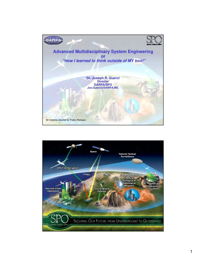
Advanced Multidisciplinary System Engineering or “How I learned to think outside of MY box!” Dr. Joseph R. Guerci Director DARPA/SPO Joe.Guerci@DARPA.MIL All material cleared for Public Release 1
Outline • Breakthrough systems/technologies are almost always multidisciplinary – Arise from cross-fertilization – “Cross-fertilization” occurs in someone’s mind • “Thinking outside the box” = “Thinking outside your box” – Examples: • KASSPER • HISS • New Trend in Multidisciplinary Systems Engineering – Level 1: System = Interconnected set of single-purpose subsystems – Level 2: System = Interconnected set of multi-purpose subsystems – Level 3: System = Embedded multi-purpose subsystems w/o clear boundaries • Example: ISIS • Summary Sample SPO Projects (A Multidisciplinary Systems Technology Office) Revolutionary Space and Near-Space Technologies Advanced Intelligent Signal Processing & Embedded Systems Next Generation Chem/Bio Sensors & Protection Nicking Enzyme Nicking Enzyme PRODUCT PRODUCT IDA IDA 3’ 3’ 3’ 5’ 5’ 5’ 3’ 3’ 5’ 5’ Pathogen DNA Pathogen DNA DNA Polymerase DNA Polymerase 5’ 5’ 3’ 3’ 5’ 5’ 3’ 3’ PRODUCT PRODUCT IRSG IRSG RNA RNA Polymerase Polymerase Pathogen RNA Pathogen RNA IAR IAR PRODUCT PRODUCT Toxin Toxin RNA RNA Polymerase Polymerase 2
mD Adaptive Signal Processing • Example: Space-Time Adaptive Processing (STAP) Space-Time Adaptive Beamformer “Ideal” Adapted Pattern Optimum Solution • Weiner-Hopf = R − 1 (Optimum space-time beamformer weights) w s (Desired signal “steering vector”) (Inverse of total interference covariance matrix) ∈ , NM w s C × ∈ NM NM R C − ~10' 100' NM s s 3
Covariance Estimation Problem • Practical implementation example and real data example (White Sands DARPA Mountain Top Radar) Sample Covariance Estimation Ideal (Stationary) Data Measured Data = ∑ x x ˆ ′ R i i ∈Ω i Welcome to the Real-World! Extremely suboptimal radar performance can occur if one or more of the following occurs: (High false alarm rates and/or low P d ) • Heterogeneous Clutter – Rapidly varying terrain • Mountainous (rapid elevation/reflectivity variation) • Rapid land cover variations (e.g., littoral) • Dense “Target” Backgrounds – “Moving Clutter” • Military/civilian vehicles • Large Discretes and “Spiky” Clutter – Urban clutter – Power lines, towers, steep mountainous terrain • Range-Varying (Nonstationary) Clutter Loci – Bi/Multistatics – Nonlinear array geometries (e.g., circular arrays) One or More of the Above is Almost Always Present in Real-World Ops! 4
Serious Performance Impacts!! (KASSPER ’02 Data Cube & APTI Data Set) SINR Loss High False Alarm Rates GMTI Range−Doppler Data (dB−thermal) rang bin 240 (38.6km) 0 60 −10 50 SINR/SNR o (dB) −20 40 Range Bin # −30 30 −40 optimal PCI−40 20 −50 MWF−40 post−Doppler (3 bin) 10 −60 −70 −0.5 −0.4 −0.3 −0.2 −0.1 0 0.1 0.2 0.3 0.4 −50 0 50 100 150 Doppler (Fraction PRF) Doppler (m/s) AMF Exceedance 0 10 STAP Only STAP w/ Pre−Whitening Rx y distance (km) −> (latitude) −1 10 50 Fraction Exceeding Value 40 −2 10 30 −3 10 20 −4 10 10 0 −5 10 0 20 40 60 80 100 −10 −5 0 5 10 15 20 25 30 Pixel SINR (dB) (35.73°,118.5°) x distance (km) −> (longitude) Knowledge-Aided Sensor Signal Processing & Expert Reasoning (KASSPER) Radar Environmental Knowledge Bases Measured Predicted (DTED/DFAD/LCLU, SAR, etc.) Bald Earth (DARPA Mtn Top) (DTED Level-1) Range Doppler KASSPER KASSPER Physical Clutter Knowledge Base Clutter Knowledge Base Clutter Knowledge Base Clutter Knowledge Base GPS/INS GPS/INS GPS/INS GPS/INS GPS/INS GPS/INS GPS/INS GPS/INS GPS/INS GPS/INS Databases Clutter Cell Returns Clutter Cell Returns Clutter Cell Returns Clutter Cell Returns Clutter Steering Vectors Clutter Steering Vectors Clutter Steering Vectors Clutter Steering Vectors { } { } { } { } { } { } { } { } γ γ γ γ C C C C i i i i i i i i Real-Time Physical = = = = γ γ γ γ 2 2 2 2 ′ ′ ′ ′ + + + + σ σ σ σ 2 2 2 2 Sensor Characteristics Sensor Characteristics Sensor Characteristics Sensor Characteristics Sensor Characteristics Sensor Characteristics Sensor Characteristics Sensor Characteristics ∑ ∑ ∑ ∑ R R R R C C C C C C C C I I I I i i i i i i i i i i i i N Elements N Elements N Elements N Elements N Elements N Elements N Elements N Elements N Elements N Elements KA KA KA KA M P M P M P M P M P M P M P M P M P M P ulse ulse ulse ulse ulse ulse ulse ulse ulse ulse s s s s s s s s s s M Pulse M Pulse M Pulse M Pulse M Pulse M Pulse M Pulse M Pulse M Pulse M Pulse s s s s s s s s s s Database T T T T T T T T T T . . . . . . . . . . T T T T T T T T T T . . . . . . . . . . . . . . . . . . . . . . . . . . . . . . T T T T T T T T T T . . . . . . . . . . T T T T T T T T T T Sum Sum Sum Sum Over Over Over Over . . . . . . . . . . . . . . . . . . . . Clutter Clutter Clutter Clutter Cells Cells Cells Cells Array S Array S Array S Array S Array S Array S Array S Array S Array S Array S napshots napshots napshots napshots napshots napshots napshots napshots napshots napshots [ x 1 [ x 1 [ x 1 [ x 1 [ x 1 [ x 1 [ x 1 [ x 1 [ x 1 [ x 1 . . . . . . . . . . x 2 x 2 x 2 x 2 x 2 x 2 x 2 x 2 x 2 x 2 x 3 • • • x M x 3 • • • x M x 3 • • • x M x 3 • • • x M x 3 • • • x M x 3 • • • x M x 3 • • • x M x 3 • • • x M x 3 • • • x M x 3 • • • x M ] . . ] ] ] ] ] . . . ] ] ] ] . . . . . -0.5 -0.5 -0.5 -0.5 20 20 1 st Stage 1 st Stage 2 nd Stage 2 nd Stage 20 20 EM Modeling 10 10 10 10 Knowledge-Aided Knowledge-Aided Conventional Conventional 0 0 0 0 Pre-Filter Response Pre-Filter Response Filter Filter -10 -10 -10 -10 Tools 0 0 0 0 -20 -20 -20 -20 -30 -30 -30 -30 -40 -40 -40 -40 -50 -50 Nonstationary Clutter Nonstationary Clutter -50 -50 Reduced-Rank Reduced-Rank 0.5 0.5 -60 -60 (plus Signal) (plus Signal) 0.5 0.5 -60 -60 -0.5 -0.5 0 0 0.5 0.5 KA Pre-Filter KA Pre-Filter -0.5 -0.5 0 0 0.5 0.5 Conventional Filter Conventional Filter 1 1 X X = = − − ˆ − ˆ − 1 1 = = 1 1 Y Y R R 2 2 X X 1 1 Z Z R R 2 2 Y Y HPEC − − ˆ − ˆ − KA KA R R 2 2 2 2 SMI SMI R R Detector Detector KA KA SMI SMI 1980 1980 2000 5
Intelligent Adaptive Radars “Real-world nonstationarity does NOT support conventional adaptivity” Space-Time Advanced and CACFAR IF Sidelobe Fully Adaptive Adaptive (STAP) Radar returns Real-Time AGC, etc. Canceler Array Radar STAP 50’s 60’s 70’s 80’s 90’s Old First Gen Statistical Signal Processing Classic knowledge-aided Real-time Reinventing Adaptive Radar 00’s 10’s Savant Knowledge KASSPER Multi-function, High-speed, slow access single function speeds FLOPS/Throughput Data type/MBytes New + KASSPER True “Intelligent” Processing VMAP Discrete SAR Roads Conventional vs. KASSPER HPEC Processing KASSPER HPEC Challenge: Conventional Highly Parallel Systolic Array Implementation Optimizing adaptation by injecting Space-Time Filtering (Achieves 100’s to 1000’s of GFLOPS) environmental knowledge . Space-Time . “intelligently” into the front-end . Snapshot signal flow Vector x Ω + 2 i First Gen Real-Time KASSPER HPEC x + 1 i ˆ ′ = ∑ Test x R x x i k k i Cell Ω x − 1 i “Guard” x Cells Ω − 2 i Intelligent . . Signal Range . Processing Cells − 1 = R w s Clutter • KASSPER requires memory • KASSPER requires memory Knowledge access interrupts access interrupts Base • Optimal interrupt • Optimal interrupt scheduling scheduling • Optimized ISP • Optimized ISP • “Look-Ahead” scheduling QR Factorization w/ Back substitution • “Look-Ahead” scheduling (from Antenna-Based Signal Processing Techniques for Radar , A. Farina, Artech House) 6
Recommend
More recommend
Explore More Topics
Stay informed with curated content and fresh updates.
