Advanced 3D-Data Structures 3D scanner: produces a set of spatial - PDF document

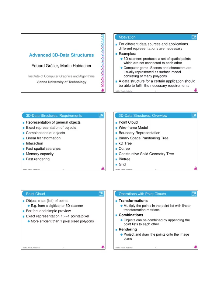
Motivation For different data sources and applications different representations are necessary Examples: Advanced 3D-Data Structures 3D scanner: produces a set of spatial points which are not connected to each other Eduard Gröller, Martin Haidacher Computer game: Scenes and characters are usually represented as surface model consisting of many polygons Institute of Computer Graphics and Algorithms A data structure for a certain application should Vienna University of Technology be able to fulfill the necessary requirements Gröller, Theußl, Haidacher 2 3D-Data Structures: Requirements 3D-Data Structures: Overview Representation of general objects Point Cloud Exact representation of objects Wire-frame Model Combinations of objects Boundary Representation Linear transformation Binary Space Partitioning Tree Interaction kD Tree Fast spatial searches Octree Memory capacity Constructive Solid Geometry Tree Fast rendering Bintree Grid Gröller, Theußl, Haidacher 3 Gröller, Theußl, Haidacher 4 Point Cloud Operations with Point Clouds Object = set (list) of points Transformations E.g. from a digitizer or 3D scanner Multiply the points in the point list with linear transformation matrices For fast and simple preview Combinations Exact representation if >=1 points/pixel Objects can be combined by appending the More efficient than 1 pixel sized polygons point lists to each other Rendering Project and draw the points onto the image plane Gröller, Theußl, Haidacher 5 Gröller, Theußl, Haidacher 6

Properties of Point Clouds Surfels (SURFace ELementS) http://www.merl.com/projects/surfels/ Advantages movies: cab, wasp, salamander with holes, Fast rendering salamander corrected (more movies on Exact representation & rendering possible web page) Fast transformations Disadvantages Many points (curved obj., exact representation) High memory consumption Limited combination operations Gröller, Theußl, Haidacher 7 QSplat (1/2) QSplat (2/2)  3D scan of 2.7 meter statue of St. Matthew at 0.25 mm  102.868.637 points  File size: 644 MB  Preprocessing time: 1 hour  Demo on laptop (PII 366, 128 MB), no 3D graphics Interactive (8 frames/sec) High quality (8 sec) hardware  http://graphics.stanford.edu/so ftware/qsplat/ Gröller, Theußl, Haidacher 9 Gröller, Theußl, Haidacher 10 3D-Data Structures: Overview Wire-Frame Model Point Cloud Object is simplified to 3D lines, each edge of the object is represented by a line in the model Wire-frame Model Boundary Representation Binary Space Partitioning Tree edge list Edge list A A B C L kD Tree B 5 3 A ........ C D Octree 8 G 2 2 E F Constructive Solid Geometry Tree H point list Vertex list K 6 4 J x1 x2 x3 x4 x5 x8 Bintree L ........ y1 y2 y3 y4 y5 y8 7 I 1 z1 z2 z3 z4 z5 z8 Grid 2 4 5 8 1 3 Gröller, Theußl, Haidacher 11 Gröller, Theußl, Haidacher 12

Operations with Wire-Frame Model Properties of Wire-Frame Models Transformations Advantages Multiply the points in the point list with linear Quick rendering transformation matrices Easy and quick transformations Combinations Generation of models via digitization Objects can be combined by appending the Disadvantages point and edge lists to each other High memory consumption Rendering Inexact (no surfaces, no occlusion) Projection of all points onto image plane and Restricted combination possibilities drawing of edges in between Curves are approximated by straight lines Gröller, Theußl, Haidacher 13 Gröller, Theußl, Haidacher 14 Boundary Representation (B-Rep) 3D-Data Structures: Overview V 2 E 6 Point Cloud E 1 V 5 E 2 Wire-frame Model S 1 V 1 S 2 E 5 Boundary Representation E 3 V 3 E 4 V 4 Binary Space Partitioning Tree vertex list edge list face list kD Tree V 1 : x 1 y 1 z 1 E 1 : V 1 V 2 S 1 : E 1 E 2 E 3 Octree V 2 : x 2 y 2 z 2 E 2 : V 2 V 3 S 2 : E 2 E 4 E 5 E 6 Constructive Solid Geometry Tree V 3 : x 3 y 3 z 3 E 3 : V 3 V 1 V 4 : x 4 y 4 z 4 E 4 : V 3 V 4 Bintree V 5 : x 5 y 5 z 5 E 5 : V 4 V 5 Grid E 6 : V 5 V 2 Gröller, Theußl, Haidacher 15 Gröller, Theußl, Haidacher 16 Lists for B-Reps (1/4) Lists for B-Reps (2/4) Face list Face list S 1 S 2 S 1 S 2 E 1 E 2 E 3 E 4 E 5 E 6 Gröller, Theußl, Haidacher 17 Gröller, Theußl, Haidacher 18

Lists for B-Reps (3/4) Lists for B-Reps (4/4) Face list Face list S 1 S 2 S 1 S 2 Edge list Vertex list x y z x y z x y z x y z x y z x y z x y z x y z x y z x y z V 1 V 2 V 3 V 4 V 5 V 1 V 2 V 3 V 4 V 5 Gröller, Theußl, Haidacher 19 Gröller, Theußl, Haidacher 20 Winged Edge Data Structure Operations with B-Reps (1/2) Alternative for normal hierarchical B-Rep Transformations Here the central element is the edge: All points are transformed as with wire-frame model, additionally surface equations or normal vectors can be transformed edge list face_cw Rendering Pstart succ_cw pred_cw Pend edge face_cw Hidden surface or hidden line algorithms can Pstart Pend face_ccw be used because the surfaces of the objects pred_cw pred_ccw succ_ccw succ_ccw are known, so that the visibility can be pred_ccw succ_ccw face_ccw calculated faces x 1st edge y 1st edge z points Gröller, Theußl, Haidacher 21 Gröller, Theußl, Haidacher 22 Operations with B-Reps (2/2) Combinations of B-Reps (1/4) Combinations Every polygon has a box enclosure  simple test if polygons can intersect 1. Split the polygons of object A at the intersections with the polygons of object B Use only convex polygons and produce only convex polygons as results 2. Split the polygons of object B at ... of A  simple intersection tests 3. Classify all polygons of A as "in B", "outside B" or "on the surface of B“ 1: 2: 4. Classify all polygons of B in the same way 5. Remove the redundant polygons of A and B   A A A B B B according to the operator and combine the remaining polygons of A and B Gröller, Theußl, Haidacher 23 Gröller, Theußl, Haidacher 24

Combinations of B-Reps (2/4) Combinations of B-Reps (3/4) A ray is traced in the direction of the normal Improvement: points of A, which lie on the vector of the polygon to be classified: surface of B, are marked as border points Ray hits no polygon of B  "outside B" during the dividing process (and vice versa)  only very few polygons have to be classified First polygon of B hit from front  "outside B" with the complex method First polygon of B hit from back  "in B" border point outside A "outside B" "in B" in B A B B B A A border point Gröller, Theußl, Haidacher 25 Gröller, Theußl, Haidacher 26 Combinations of B-Reps (4/4) Requirements on B-Reps for this Alg. No open (non-closed) objects Polygons can be removed according to tables: Only convex polygons in B outside B on B (coplanar) For op. NV equal different No double points polygons yes no no yes A or B Additional links in the vertex list between of A A and B no yes no yes neighbor points with equal classification yes no yes no A sub B x1 x2 x3 x4 x5 x5 xn ........ in A outside A on A (coplanar) y1 y2 y3 y4 y5 y5 yn For z1 z2 z3 z4 z5 z5 zn op. NV equal different vertex list polygons yes no yes yes A or B of B no yes yes yes A and B A sub B no yes yes yes Gröller, Theußl, Haidacher 27 Gröller, Theußl, Haidacher 28 Partitioning of Object Surfaces Tesselation Necessary to approximate curved surfaces Divide polygons in smaller polygons (triangles) until the approximation is exact enough Surfaces that can be parameterized: Normal vector criterion as termination condition: E.g. free form surfaces, quadrics, N 1  2  1–  superquadrics partitioning of parameter space, one patch for Normal vectors of neighboring polygons are similar: every 2D parameter interval Surfaces that cannot be parameterized: N 2 N 1 Objekt E.g. implicit surfaces, "bent" polygons Approximation  tesselation, subdivision surfaces Gröller, Theußl, Haidacher 29 Gröller, Theußl, Haidacher 30