Admixture of Poisson MRFs (APM): A Topic Model with Word - PowerPoint PPT Presentation
Admixture of Poisson MRFs (APM): A Topic Model with Word Dependencies David Inouye*, Pradeep Ravikumar, Inderjit Dhillon Tuesday, June 24, 2014 * Presenter David Inouye*, Pradeep Ravikumar, Inderjit Dhillon Admixture of Poisson MRFs (ICML
Admixture of Poisson MRFs (APM): A Topic Model with Word Dependencies David Inouye*, Pradeep Ravikumar, Inderjit Dhillon Tuesday, June 24, 2014 * Presenter David Inouye*, Pradeep Ravikumar, Inderjit Dhillon Admixture of Poisson MRFs (ICML 2014, Beijing, China)
k Multinomials “Fine Arts” “Fine Arts” “Temperature” “Fine Arts” theater theater nuclear theater Independent Models music music heat music plays plays sun plays LDA, PLSA, SAM, etc. novels novels temperature novels Document Corpus life life soviet life Doc. 4 - Music is an art form Doc. 4 - Music is an art form Doc. 1 - Nuclear power, or Doc. 4 - Music is an art form whose medium is sound and whose medium is sound and nuclear energy, is the use of whose medium is sound and silence… silence… exothermic nuclear processes... silence… k Poisson MRFs Doc. 4 - Music is an art form Doc. 4 - Music is an art form Doc. 4 - Music is an art form Doc. 2 - Theatre or theater is a whose medium is sound and whose medium is sound and whose medium is sound and collaborative form of fine art that silence… silence… silence… uses live performers ... Doc. 4 - Music is an art form Doc. 4 - Music is an art form Doc. 4 - Music is an art form Doc. 3 - A temperature is a whose medium is sound and whose medium is sound and whose medium is sound and numerical measure of hot or cold. silence… silence… silence… Its measurement is…. Doc. 4 - Music is an art form Doc. 4 - Music is an art form Doc. 4 - Music is an art form whose medium is sound and whose medium is sound and whose medium is sound and silence… silence… silence… Dependent Model Admixture of Poisson MRFs Possible applications: - Topic Visualization - Corpus Summarization - Word Sense Disambiguation - Semantic Similarity - Document Classification ◮ Previous topic models assume independence between words. ◮ An Admixture of Poisson MRFs (APM), however, explicitly models word dependencies . David Inouye*, Pradeep Ravikumar, Inderjit Dhillon Admixture of Poisson MRFs (ICML 2014, Beijing, China)
Main Contributions 1. Generalized Admixtures 2. (Background) Poisson MRF [Yang et al. 2012]) ◮ Poisson MRFs in the context of LDA ◮ Novel conjugate prior for a Poisson MRF 3. Admixture of Poisson MRFs (APM) 4. Tractable MAP parameter estimation David Inouye*, Pradeep Ravikumar, Inderjit Dhillon Admixture of Poisson MRFs (ICML 2014, Beijing, China)
Formalizing Generalized Admixtures ◮ Mixtures - Draws from single x 2 Mixture component distribution. (Top) "Documents" Components ◮ Admixtures - Draws from a distribution whose parameters are a convex combination of component parameters. (Bottom) x 1 k ˛ “ φ = Ψ − 1 h i” ˛ ¯ X w j Ψ( φ j ) Admix. ( x | w , Φ) = Pr Pr x ˛ x 2 Base Sparse j =1 Dense "Document" "Topic" ◮ Examples of different Ψ Sparse k "Topic" “ ˛ w j λ j ” ˛ ¯ Dense Admix. ( x | w , λ 1 ... k ) = Pr X Pr x λ = ˛ "Document” Poiss. j =1 x 1 k “ ˛ ´” Admix. ( x | w , λ 1 ... k ) = Pr ˛ ¯ X w j ln ( λ j ) ` Pr x λ = exp ˛ Poiss. j =1 David Inouye*, Pradeep Ravikumar, Inderjit Dhillon Admixture of Poisson MRFs (ICML 2014, Beijing, China)
Examples of Admixture Models 1. LDA [Blei et al. 2003] ◮ LDA is an admixture of Multinomials (i.e. Mult( p 1 ), Mult( p 2 ), · · · , Mult( p k )) ◮ Dirichlet prior over p 1 ... k 2. Population Admixtures ◮ Equivalent model to LDA in genetics [Pritchard et al. 2000] ◮ Admixture term comes from genetics literature ◮ Original ancestors of population correspond to “topics” ◮ Individuals of a population correspond to “documents” 3. Spherical Admixture Model [Reisinger et al. 2010] ◮ Von Mises-Fisher base distribution (an independent Gaussian analog on unit hypersphere) ◮ Von Mises-Fisher priors David Inouye*, Pradeep Ravikumar, Inderjit Dhillon Admixture of Poisson MRFs (ICML 2014, Beijing, China)
Background: Poisson MRFs [Yang et al., 2012] If we assume the node conditional distributions are Poisson, P(A | B, C) P(B | A, C) P(C | A, B) P(A, B, C) ?? does there exist a joint MRF distribution that has these conditionals? ◮ Poisson MRF joint distribution: � � p � θ T x + x T Θ x − PMRF ( x | θ , Θ) ∝ exp Pr ln ( x s !) . s =1 ◮ Node conditionals are 1-D Poissons: Pr( x s | x − s , θ s , Θ s ) ∝ exp { ( θ s + x T Θ s ) x s − ln ( x s !) } . � �� � η s David Inouye*, Pradeep Ravikumar, Inderjit Dhillon Admixture of Poisson MRFs (ICML 2014, Beijing, China)
Independent PMRF Positive Dependency PMRF 8 8 Count of Word 2 Count of Word 2 6 6 4 4 2 2 0 0 0 2 4 6 8 0 2 4 6 8 Count of Word 1 Count of Word 1 Negative Dependency PMRF 1. Each conditional (”slice”) 8 of a PMRF is 1-D Poisson. Count of Word 2 6 2. Distinct from Gaussian MRF 4 3. Positive dependencies can 2 model word co-occurence . a 0 a See [Yang et al. 2013] for SPMRF model that 0 2 4 6 8 Count of Word 1 allows for positive dependencies. David Inouye*, Pradeep Ravikumar, Inderjit Dhillon Admixture of Poisson MRFs (ICML 2014, Beijing, China)
Poisson MRFs in the Context of LDA ◮ LDA uses Multinomial distributions but if the parameter x = � p λ = � p s =1 x s | ˜ N ∼ Poisson(˜ s =1 λ ), then the joint distribution is an independent Poisson model: 1 � � � � x | ˜ x | θ = ( λ 1 , · · · , λ p ) / ˜ Pr ˜ λ Pr λ, N = ˜ x Poiss Mult p = e − ˜ � λ s � x s λ x ! ˜ � ˜ λ ˜ x � p ˜ x ! ˜ s =1 x s ! λ s =1 � ˜ � x s p e − ˜ λ = ˜ x ! λλ s � � p ˜ x ! ˜ s =1 x s ! λ s =1 p e − λ s � x s ! λ x s = Ind. Poiss ( x | λ 1 , · · · , λ p ) = Pr s s =1 ◮ Therefore, the topic-word distribution of LDA can be viewed as a special case of a Poisson MRF . 1 Gopalan et al. (2013) recently introduced the connection between LDA and independent Poissons in the context of matrix factorization. David Inouye*, Pradeep Ravikumar, Inderjit Dhillon Admixture of Poisson MRFs (ICML 2014, Beijing, China)
Novel conjugate prior for a Poisson MRF ◮ Form of a conjugate prior: Pr( θ , Θ) ∝ exp { β T θ + β T Θ β − γ A ( θ , Θ) − λ θ � θ � 2 2 − λ � vec(Θ) � 1 } , where A ( θ , Θ) is the log partition function of a PMRF. 2 ◮ λ � vec(Θ) � 1 term encourages sparsity in Θ (i.e. a Laplace prior on Θ) . ◮ β can be viewed as adding pseudo-counts (similar to a Dirichlet prior for a Multinomial) 2 λ θ � θ � 2 2 and λ � vec(Θ) � 1 needed for normalization of this prior distribution. In practice, λ θ can be set arbitrarily small and is thus ignored in subsequent discussion. David Inouye*, Pradeep Ravikumar, Inderjit Dhillon Admixture of Poisson MRFs (ICML 2014, Beijing, China)
Admixture of Poisson MRFs (APM) ◮ Poisson MRF base distribution ◮ Priors ◮ Dirichlet prior on admixture weights ◮ Conjugate prior on component PMRFs APM ( x , w , θ 1 ... k , Θ 1 ... k ) Pr ˛ k k ! k ˛ ¯ X w j θ j , ¯ X w j Θ j Y Pr( θ j , Θ j ) = Pr x θ = Θ = Pr Dir ( w ) ˛ ˛ PMRF ˛ j =1 j =1 j =1 ◮ Topics → graphs over words (from PMRF parameters) ◮ Documents → weights over topics (dimensionality reduction) David Inouye*, Pradeep Ravikumar, Inderjit Dhillon Admixture of Poisson MRFs (ICML 2014, Beijing, China)
Parameter Estimation using Approximate Posterior ◮ Because the Poisson MRF likelihood does not have a closed-form solution, we approximate the likelihood with the pseudo log-likelihood : L ≈ ˆ L ( X | W , θ 1 ... k , Θ 1 ... k ) n p � � = η is x is − ln ( x is !) − A ( η is ) , � �� � s =1 i =1 Conditional Poisson log-likelihood where η is = � k j =1 w ij ( θ j i Θ j s + x T s ) is the canonical parameter of a univariate Poisson (i.e. λ is = exp( η is )). David Inouye*, Pradeep Ravikumar, Inderjit Dhillon Admixture of Poisson MRFs (ICML 2014, Beijing, China)
Tractable MAP Parameter Estimation ◮ The approximate log posterior is: P (W , θ 1 ... k , Θ 1 ... k | X ) ≈ ˆ L × ln (priors) n p k � � � +( α − 1) T ln ( w i ) λ � Θ j � 1 ∝ η is ( x is + β s ) − ( γ +1)A ( η is ) − i =1 s =1 � �� � � �� � j =1 psuedo-counts Dirichlet prior � �� � ℓ 1 penalty for sparsity ◮ A MAP parameter estimate can be computed by the following: k � W , θ 1 ... k , Θ 1 ... k − f (W , θ 1 ... k , Θ 1 ... k ) � Θ j � 1 arg min + δ W (W) + λ j =1 � �� � � �� � differentiable nonsmooth but convex ◮ A proximal gradient method can used David Inouye*, Pradeep Ravikumar, Inderjit Dhillon Admixture of Poisson MRFs (ICML 2014, Beijing, China)
Recommend
More recommend
Explore More Topics
Stay informed with curated content and fresh updates.


