Adaptive treatment assignment in experiments for policy choice - PowerPoint PPT Presentation
Adaptive treatment assignment in experiments for policy choice Maximilian Kasy Anja Sautmann January 20, 2020 Introduction The goal of many experiments is to inform policy choices: 1. Job search assistance for refugees: Treatments:
Adaptive treatment assignment in experiments for policy choice Maximilian Kasy Anja Sautmann January 20, 2020
Introduction The goal of many experiments is to inform policy choices: 1. Job search assistance for refugees: • Treatments: Information, incentives, counseling, ... • Goal: Find a policy that helps as many refugees as possible to find a job. 2. Clinical trials : • Treatments: Alternative drugs, surgery, ... • Goal: Find the treatment that maximizes the survival rate of patients. 3. Online A/B testing : • Treatments: Website layout, design, search filtering, ... • Goal: Find the design that maximizes purchases or clicks. 4. Testing product design : • Treatments: Various alternative designs of a product. • Goal: Find the best design in terms of user willingness to pay. 1 / 35
Example • There are 3 treatments d . • d = 1 is best, d = 2 is a close second, d = 3 is clearly worse. (But we don’t know that beforehand.) • You can potentially run the experiment in 2 waves. • You have a fixed number of participants. • After the experiment, you pick the best performing treatment for large scale implementation. How should you design this experiment? 1. Conventional approach. 2. Bandit approach. 3. Our approach. 2 / 35
Conventional approach Split the sample equally between the 3 treatments, to get precise estimates for each treatment. • After the experiment, it might still be hard to distinguish whether treatment 1 is best, or treatment 2. • You might wish you had not wasted a third of your observations on treatment 3, which is clearly worse. The conventional approach is 1. good if your goal is to get a precise estimate for each treatment. 2. not optimal if your goal is to figure out the best treatment. 3 / 35
Bandit approach Run the experiment in 2 waves split the first wave equally between the 3 treatments. Assign everyone in the second (last) wave to the best performing treatment from the first wave. • After the experiment, you have a lot of information on the d that performed best in wave 1, probably d = 1 or d = 2, • but much less on the other one of these two. • It would be better if you had split observations equally between 1 and 2. The bandit approach is 1. good if your goal is to maximize the outcomes of participants. 2. not optimal if your goal is to pick the best policy. 4 / 35
Our approach Run the experiment in 2 waves split the first wave equally between the 3 treatments. Split the second wave between the two best performing treatments from the first wave. • After the experiment you have the maximum amount of information to pick the best policy. Our approach is 1. good if your goal is to pick the best policy, 2. not optimal if your goal is to estimate the effect of all treatments, or to maximize the outcomes of participants. Let θ d denote the average outcome that would prevail if everybody was assigned to treatment d . 5 / 35
What is the objective of your experiment? 1. Getting precise treatment effect estimators, powerful tests: � θ d − θ d ) 2 (ˆ minimize d ⇒ Standard experimental design recommendations. 2. Maximizing the outcomes of experimental participants: � θ D i maximize i ⇒ Multi-armed bandit problems. 3. Picking a welfare maximizing policy after the experiment: maximize θ d ∗ , where d ∗ is chosen after the experiment. ⇒ This talk. 6 / 35
Preview of findings • Adaptive designs improve expected welfare. • Features of the optimal treatment assignment: • Shift toward better performing treatments over time. • But don’t shift as much as for Bandit problems: We have no “exploitation” motive! • Asymptotically: Equalize power for comparisons of each suboptimal treatment to the optimal one. • Fully optimal assignment is computationally challenging in large samples. • We propose a simple exploration sampling algorithm. • Prove theoretically that it is rate-optimal for our problem, because it equalizes power across suboptimal treatments. • Show that it dominates alternatives in calibrated simulations. 7 / 35
Literature • Adaptive designs in clinical trials: • Berry (2006), FDA (2018). • Bandit problems: • Gittins index (optimal solution to some bandit problems): Weber (1992). • Regret bounds for bandit problems: Bubeck and Cesa-Bianchi (2012). • Thompson sampling: Russo et al. (2018). • Best arm identification: • Rate-optimal (oracle) assignments: Glynn and Juneja (2004). • Poor rates of bandit algorithms: Bubeck et al. (2011), • Bayesian algorithms: Russo (2016). Key references for our theory results. • Empirical examples for our simulations: • Ashraf et al. (2010), • Bryan et al. (2014), • Cohen et al. (2015). 8 / 35
Setup Thompson sampling and exploration sampling The rate optimal assignment Exploration sampling is rate optimal Calibrated simulations Implementation in the field Covariates and targeting
Setup • Waves t = 1 , . . . , T , sample sizes N t . • Treatment D ∈ { 1 , . . . , k } , outcomes Y ∈ { 0 , 1 } . • Potential outcomes Y d . • Repeated cross-sections: ( Y 0 it , . . . , Y k it ) are i.i.d. across both i and t . • Average potential outcome: θ d = E [ Y d it ] . • Key choice variable: Number of units n d t assigned to D = d in wave t . • Outcomes: Number of units s d t having a “success” (outcome Y = 1). 9 / 35
Treatment assignment, outcomes, state space • Treatment assignment in wave t : n t = ( n 1 t , . . . , n k t ) . • Outcomes of wave t : s t = ( s 1 t , . . . , s k t ) . • Cumulative versions: � � � M t = N t ′ , m t = n t , r t = s t . t ′ ≤ t t ′ ≤ t t ′ ≤ t • Relevant information for the experimenter in period t + 1 is summarized by m t and r t . • Total trials for each treatment, total successes. 10 / 35
Design objective and Bayesian prior • Policy objective θ d ∗ T . • where d ∗ T is chosen after the experiment. • Prior • θ d ∼ Beta ( α d 0 , β d 0 ), independent across d . • Posterior after period t : θ d | m t , r t ∼ Beta ( α d t , β d t ) α d t = α d 0 + r d t β d t = β d 0 + m d t − r d t . • Posterior expected social welfare as a function of d : SW T ( d ) = E [ θ d | m T , r T ] , α d T = , α d T + β d T d ∗ T ∈ argmax SW T ( d ) . d 11 / 35
Regret • True optimal treatment: d (1) ∈ arg max d ′ θ d ′ . • Policy regret when choosing treatment d : ∆ d = θ d (1) − θ d . • Maximizing expected social welfare is equivalent to minimizing the expected policy regret at T , E [∆ d | m T , r T ] = θ d (1) − SW T ( d ) • In-sample regret : Objective considered in the bandit literature, � 1 ∆ D it . M i , t Different from policy regret ∆ d ∗ T ! 12 / 35
Setup Thompson sampling and exploration sampling The rate optimal assignment Exploration sampling is rate optimal Calibrated simulations Implementation in the field Covariates and targeting
Thompson sampling • Thompson sampling • Old proposal by Thompson (1933). • Popular in online experimentation. • Assign each treatment with probability equal to the posterior probability that it is optimal. � � θ d ′ | m t − 1 , r t − 1 p d t = P d = argmax . d ′ • Easily implemented: Sample draws � θ it from the posterior, assign ˆ θ d D it = argmax it . d • Expected Thompson sampling • Straightforward modification for the batched setting. • Assign non-random shares p d t of each wave to treatment d . 13 / 35
Exploration sampling • Agrawal and Goyal (2012) proved that Thompson-sampling is rate-optimal for the multi-armed bandit problem. • It is not for our policy choice problem! • We propose the following modification. • Exploration sampling : Assign shares q d t of each wave to treatment d , where q d t = S t · p d t · (1 − p d t ) , 1 S t = � t ) . d p d t · (1 − p d • This modification 1. yields rate-optimality (theorem coming up), and 2. improves performance in our simulations. 14 / 35
Illustration of the mapping from Thompson to exploration sampling 1.00 0.75 0.50 0.25 0.00 p q p q p q p q 15 / 35
Setup Thompson sampling and exploration sampling The rate optimal assignment Exploration sampling is rate optimal Calibrated simulations Implementation in the field Covariates and targeting
The rate-optimal assignment: Lemma 1 T = 1+ r d Denote the estimated success rate of d at time T by ˆ θ d T T . 2+ m d The rate of convergence to zero of expected policy regret � � � ∆ d · P θ d ′ ˆ R(T) = argmax T = d d ′ d is equal to the slowest rate of convergence Γ d across d � = d (1) for the probability of d being estimated to be better than d (1) . Lemma • Assume that the optimal policy d (1) is unique. Suppose that for all d � � T →∞ − 1 θ d (1) θ d ˆ T > ˆ = Γ d . lim NT log P T • Then � � − 1 d � = d (1) Γ d . lim NT log R(T) = min T →∞ 16 / 35
Recommend
More recommend
Explore More Topics
Stay informed with curated content and fresh updates.
