Abstract Machines What is an abstract machine? - a set of legal - PowerPoint PPT Presentation
Concepts of Program Design Abstract Machines Gabriele Keller Ron Vanderfeesten Abstract Machines What is an abstract machine? - a set of legal states final and initial states as subset - A set of instructions altering the state of the
Concepts of Program Design Abstract Machines Gabriele Keller Ron Vanderfeesten
Abstract Machines • What is an abstract machine? - a set of legal states ‣ final and initial states as subset - A set of instructions altering the state of the machine ‣ it should be possible to implement the operations on a real machine in a finite (preferably constant) number of steps • Why use abstract machines at all? - specifies the semantics of a programming languages - facilitates porting to other architectures - mobile code (e.g., Java Virtual Machine) • We have seen this before - similar to SOS, but with Abstract Machines, we care about performance
Control Flow • Base line: the M-machine - small step semantics for MinHs - transition system embodies essentially a very high-level (= concise, but inefficient) abstract machine - we call it the M-machine • Characteristics of the M-machine - substitution as “machine operation” ‣ why is that bad? ‣ can be avoided by using an environment - control-flow is not explicit ‣ the search rules determine next subexpression to be evaluated ‣ why is that bad?
Control Flow • Example: (Plus (Num n) (Num m)) ↦ Num (n+m) e 1 ↦ e 1 ’ (Plus e 1 e 2 ) ↦ ( Plus e 1 ’ e 2 ) e 2 ↦ e 2 ’ (Plus(Num n) e 2 ) ↦ ( Plus (Num n) e 2 ’ ) Plus(Num 3)(Num 2) ↦ Num 5 Plus(Plus(Num 3)(Num 2))(Num 4) ↦ Plus(Num 5)(Num 4) Plus(Plus(Plus(Num 3)(Num 2))(Num 4))(Num 6) ↦ Plus(Plus(Num 5)(Num 4))(Num 6) depending on the size & nesting depth of the expression, searching for the next reducible subexpression can be very expensive!!!
Control Flow • Single-step evaluation in Haskell: eval(Num n) = Num n eval e = eval (single e) single (Plus (Num n1) (Num n2)) = Num (n1 + n2) single (Plus (Num n1) e) = Plus (Num n1) (single e) single (Plus e1 e2) = Plus (single e1) e2 single (Times .... ‣ Properties: ‣ for each step, the expression has to be traversed to find the next subexpression that has to be evaluated ‣ makes heavy use of the runtime stack
The C-machine • Explicit control flow: C-machine - explicit stack - explicit handling of control flow - variable binding still handled by substitution - we call this machine the C-machine • Machine state - the current expression (as before) - a control stack of subcomputations (frames) which have to be performed before the machine terminates • Initial and final states - initial states: closed expression and an empty stack - final states: expression is a value and the stack is empty
The C-machine • Example: addition in three stages 1. Evaluate first argument ‣ first argument becomes current expression ‣ remember to continue with computation, result as first argument 2. Evaluate second argument ‣ second argument becomes current expression ‣ remember to continue with computation, result as second argument 3. Perform addition
The C-machine • How can we denote a stack frame as a term? • We use terms with holes; e.g., Plus ☐ e 2 ‣ suspended computation of addition ‣ waits for the value of its first argument • Inductive definition of frames: e expr (Plus ☐ e ) frame Plus e 1 ☐ not a frame, because first argument is v value evaluated first! (Plus v ☐ ) frame
Inductive Definition of Frames • Addition e expr (Plus ☐ e ) frame v value (Plus v ☐ ) frame • If-expressions e 1 expr e 2 expr (If ☐ e 1 e 2 ) frame • Application e expr (Apply ☐ e ) frame v value (Apply v ☐ ) frame
Stack and Machine Modes • Stacks: f 1 ▷ f 2 ▷ ◦ - f 1 is the top-most frame - f 2 is the second frame - ◦ is the empty stack • Inductive definition: ◦ stack f frame s stack f ▷ s stack • Machine modes: the C-machine operates in two modes: ‣ s ≻ e : evaluate expression e under stack s ‣ s ≺ v : return value v to stack s
Transition Rules for MinHs • Values (integers, booleans, functions) s ≻ v ↦ c s ≺ v { evaluate the value v under stack s • Addition s ≻ ( Plus e 1 e 2 ) ↦ c (Plus ☐ e 2 ) ▷ s ≻ e 1 (Plus ☐ e 2 ) ▷ s ≺ v ↦ c (Plus v ☐ ) ▷ s ≻ e 2 (Plus(Num n 1 ) ☐ ) ▷ s ≺ Num n 2 ↦ c s ≺ Num( n 1 + n 2 )
Transition Rules for MinHs • if-expressions s ≻ ( If e 1 e 2 e 3 ) ↦ c (If ☐ e 2 e 3 ) ▷ s ≻ e 1 (If ☐ e 2 e 3 ) ▷ s ≻ e 1 (If ☐ e 2 e 3 ) ▷ s ≺ True ↦ c s ≻ e 2 (If ☐ e 2 e 3 ) ▷ s ≺ False ↦ c s ≻ e 3
Transition Rules for MinHs • Function application (Apply ☐ e 2 ) ▷ s ≻ e 1 s ≻ ( Apply e 1 e 2 ) ↦ c (Apply ☐ e 2 ) ▷ s ≺ v ↦ c (Apply v ☐ ) ▷ s ≻ e 2 (Apply(Fun τ 1 τ 2 f.x.e ) ☐ ) ▷ s ≺ v ↦ c s ≻ e [ f:= ( Fun τ 1 τ 2 ( f.x.e) ) , x := v ] writing Fun instead of Recfun from now on to save some space • Observations; ‣ all the inference rules are axioms! ‣ the definition of single-step evaluation in the C-machine is not recursive ‣ the full evaluator is tail recursive (can be implemented using a while-loop)
Environments • Now, let’s get rid of substitution! • We used an environment for TinyC - but we can’t just pass it along, because we wouldn’t know when to delete bindings (Apply(Fun τ 1 τ 2 f.x.e ) ☐ ) ▷ s ≺ v ↦ c s ≻ e [ f := Fun τ 1 τ 2 f.x.e ) , x:= v ] - we need to save the old environment somewhere, and restore it when returning from the function call - can we use the stack to keep track of the environment?
The E-machine • In the E-machine ‣ we have frames defined exactly as before ‣ explicit environments, which are a sequence of variable bindings η env ● env x = v, η env ‣ stacks in the E-machine are sequences of environments and frames f frame s stack η env s stack ◦ stack η ▷ s stack f ▷ s stack ‣ states in the E-machine include an environment s | η ≻ e s | η ≺ v
The E-machine: Transition Rules • Free variables: s | η ≻ x ↦ E s | η ≺ v , if x=v ∈ η • Application: (Apply(Fun τ 1 τ 2 f.x .e ) ☐ ) ▷ s | η ≺ v ↦ E η ▷ s | f = (Fun τ 1 τ 2 f.x.e ) , x = v, η ≻ e • Returning values: η ▷ s | η ’ ≺ v ↦ E s | η ≺ v ,
The E-machine: Transition Rules • Are these rules correct? ‣ let’s look at two example usages • Example ‣ simple function application Apply(Fun Int Int ( f.x . (Plus x 1)) 3 ‣ nested application (corresponds to a function which accepts two arguments and returns the first one) Apply (Apply (Fun(Int →I nt) Int ( f.x . (Fun int int g.y.x )) 3) 1) We omit the type information, and abbreviate apply to app and write n instead of (Num n)
Example 1 ◦ | ● ≻ App(Fun( f.x .( Plus x 1)) 3) ↦ E (App ☐ 3) ▷ ◦ | ● ≻ Fun( f.x . (Plus x 1)) ↦ E (App ☐ 3) ▷ ◦ | ● ≺ Fun( f.x . (Plus x 1)) ↦ E (App(Fun( f.x . (Plus x 1)) ☐ ) ▷ ◦ | ● ≻ 3 ↦ E (App(Fun( f.x . (Plus x 1)) ☐ ) ▷ ◦ | ● ≺ 3 ↦ E ● ▷ ◦ | x = 3 , f= Fun( f.x . (Plus x 1)) , ● ≻ (Plus x 1) ↦ E (Plus ☐ 1) ▷ ● ▷ ◦ | x = 3 , f= Fun( f.x . Plus x 1) , ● ≻ x ↦ E (Plus ☐ 1) ▷ ● ▷ ◦ | x = 3 , f= Fun( f.x . Plus x 1) , ● ≺ 3 ↦ E (Plus 3 ☐ ) ▷ ● ▷ ◦ | x = 3 , f= Fun( f.x . Plus x 1) , ● ≻ 1 ↦ E (Plus 3 ☐ ) ▷ ● ▷ ◦ | x = 3 , f= Fun( f.x . Plus x 1) , ● ≺ 1 ↦ E ● ▷ ◦ | x = 3 , f= Fun( f.x . Plus x 1) , ● ≺ 4 ↦ E ◦ | ● ≺ 4
Example 2 (recfun f x = recfun g y = x) 3 4 (App(App(Fun( f.x . Fun( g.y.x )) 3) 4)
Example 2 ◦ | ● ≻ (App(App(Fun( f.x . Fun( g.y.x )) 3) 4) ↦ E (App ☐ 4) ▷ ◦ | ● ≻ (App(Fun( f.x . Fun( g.y.x )) 3) ↦ E (App ☐ 3) ▷ (App ☐ 4) ▷ ◦ | ● ≻ (Fun( f.x . fun( g.y.x )) ↦ E (App ☐ 3) ▷ (App( ☐ ,4) ▷ ◦ | ● ≺ (Fun( f.x . Fun( g.y.x )) ↦ E ... ↦ E ↦ E (App(Fun( f.x . Fun( g.y.x )) ☐ ) ▷ (App ☐ 4) ▷ ◦ | ● ≺ 3 ↦ E ● ▷ (App ☐ 4) ▷ ◦ | x = 3 , f= Fun( f.x . Fun...), ● ≻ Fun( g.y.x ) ↦ E ● ▷ (App ☐ 4) ▷ ◦ | x = 3 , f= Fun( f.x . Fun...), ● ≺ Fun( g.y.x ) ↦ E (App ☐ 4) ▷ ◦ | ● ≺ Fun( g.y.x ) ↦ E (App(Fun( g.y.x )) ☐ ) ▷ ◦ | ● ≻ 4 ↦ E (App(Fun( g.y.x )) ☐ ) ▷ ◦ | ● ≺ 4 ↦ E ◦ | y = 4 , g= Fun( g.y . x ), ● ≺ x
Dealing with partial application • Something went wrong! - returning the function value and restoring the old (empty) environment, we threw away the binding for the variable x - it now occurs freely in g ! • Problem: functions as results are not handled correctly! - free variables in the function bodies escape the environment they are defined in. - partial applications fails let f x y = x + y g = f 3 in let x = 5 in g x
Dealing with partial application • Solution: - we need to bundle returned functions with current environment - we call this a closure - requires a new form of return values: environment which 《 η , (Fun τ 1 τ 2 f.x .e ) 》 was current when function value was created - Closures only appear as values during execution - there is no source form
Transition Rules • Returning values: η ▷ s | η ’ ≻ (Num n) ↦ E s | η ≺ (Num n) s | η ≻ (Fun τ 1 τ 2 f.x .e ) ↦ E s | η ≺ 《 η , (Fun τ 1 τ 2 f.x .e ) 》 η ▷ s | η ’ ≺ v ↦ E s | η ≺ v • Application of functions: (Apply 《 η ’, (Fun τ 1 τ 2 f.x .e ) 》 ☐ ) ▷ s | η ≺ v ↦ E η ▷ s | f = (Fun τ 1 τ 2 f.x.e ) , x = v, η ’ ≻ e restore environment from closure, add binding for argument x and function f
Recommend
More recommend
Explore More Topics
Stay informed with curated content and fresh updates.
