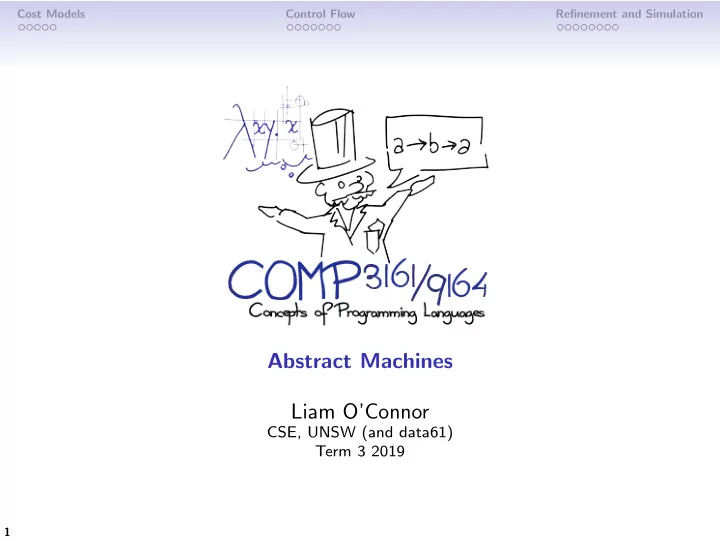
Abstract Machines Liam OConnor CSE, UNSW (and data61) Term 3 2019 - - PowerPoint PPT Presentation

Cost Models Control Flow Refinement and Simulation

Abstract Machines Liam O’Connor

CSE, UNSW (and data61) Term 3 2019

1

Cost Models Control Flow Refinement and Simulation

Big O

We all know that MergeSort has O(n log n) time complexity, and that BubbleSort has O(n2) time complexity, but what does that actually mean? Big O Notation Given functions f , g : R → R, f ∈ O(g) if and only if there exists a value x0 ∈ R and a coefficient m such that: ∀x > x0. f (x) ≤ m · g(x) What is the codomain of f ? When analysing algorithms, we don’t usually time how long they take to run on a real machine.

2

Cost Models Control Flow Refinement and Simulation

Cost Models

A cost model is a mathematical model that tries to measure of the cost of executing a program. There exist denotational cost models, that assign a cost directly to syntax: [ [·] ] : Program → Cost However in this course we will focus on operational cost models. Operational Cost Models First, we define a program-evaluating abstract machine. We can determine the time cost by counting the number of steps taken by the abstract machine.

3

Cost Models Control Flow Refinement and Simulation

Abstract Machines

Abstract Machines An abstract machine consists of:

1

A set of states Σ,

2

A set of initial states I ⊆ Σ,

3

A set of final states F ⊆ Σ, and

4

A transition relation → ⊆ Σ × Σ. We’ve seen this before in structural operational (or small-step) semantics.

4

Cost Models Control Flow Refinement and Simulation

The M Machine

Is just our usual small-step rules: e1 →M e′

1

(Plus e1 e2) →M (Plus e′

1 e2) · · ·

e1 →M e′

1

(If e1 e2 e3) →M (If e′

1 e2 e3)

(If (Lit True) e2 e3) →M e2 (If (Lit False) e2 e3) →M e3 e1 →M e′

1

(Apply e1 e2) →M (Apply e′

1 e2)

e2 →M e′

2

(Apply (Recfun (f .x. e)) e2) →M (Apply (Recfun (f .x. e)) e′

2)

v ∈ F (Apply (Recfun (f .x. e)) v) →M e[x := v, f := (Recfun (f .x. e))] The M Machine is unsuitable as a basis for a cost model. Why?

5

Cost Models Control Flow Refinement and Simulation

Performance

One step in our machine should always only be O(1) in our language implementation. Otherwise, counting steps will not get an accurate description of the time cost. This makes for two potential problems:

1

Substitution occurs in function application, which is potentially O(n) time.

2

Control Flow is not explicit – which subexpression to reduce is found by recursively descending the abstract syntax tree each time. eval (Num n) = n eval e = eval (oneStep e)

• neStep (Plus (Num n) (Num m))

= Num (n + m)

• neStep (Plus (Num n) e2)

= Plus (Num n) (oneStep e2)

• neStep (Plus e1 e2)

= Plus (oneStep e1) e2 . . .

6

Cost Models Control Flow Refinement and Simulation

The C Machine

We want to define a machine where all the rules are axioms, so there can be no recursive descent into subexpressions. How is recursion typically implemented? Stacks!

• Stack

f Frame s Stack f ⊲ s Stack Key Idea: States will consist of a current expression to evaluate and a stack of computational contexts that situate it in the overall

• computation. An example stack would be:

(Plus 3 ) ⊲ (Times (Num 2)) ⊲ ◦ This represents the computational context: (Times (Plus 3 ) (Num 2))

7

Cost Models Control Flow Refinement and Simulation

The C Machine

Our states will consist of two modes:

1

Evaluate the current expression within stack s, written s ≻ e.

2

Return a value v (either a function, integer, or boolean) back into the context in s, written s ≺ v. Initial states are those that start evaluating an expression from an empty stack, i.e. ◦ ≻ e. Final states are those that return a value to the empty stack, i.e. ◦ ≺ v. Stack frames are expressions with holes or values in them: e2 Expr (Plus e2) Frame v1 Value (Plus v1 ) Frame · · ·

8

Cost Models Control Flow Refinement and Simulation

Evaluating

There are three axioms about Plus now: When evaluating a Plus expression, first evaluate the LHS: s ≻ (Plus e1 e2) →C (Plus e2) ⊲ s ≻ e1 Once it is evaluated, switch to the RHS: (Plus e2) ⊲ s ≺ v1 →C (Plus v1 ) ⊲ s ≻ e2 Once it is evaluated, return the sum: (Plus v1 ) ⊲ s ≺ v2 →C s ≺ v1 + v2 We also have a single rule about Num that just returns the value: s ≻ (Num n) →C s ≺ n

9

Cost Models Control Flow Refinement and Simulation

Example

• ≻ (Plus (Plus (Num 2) (Num 3)) (Num 4))

→C (Plus (Num 4)) ⊲ ◦ ≻ (Plus (Num 2) (Num 3)) →C (Plus (Num 3)) ⊲ (Plus (Num 4)) ⊲ ◦ ≻ (Num 2) →C (Plus (Num 3)) ⊲ (Plus (Num 4)) ⊲ ◦ ≺ 2 →C (Plus 2 ) ⊲ (Plus (Num 4)) ⊲ ◦ ≻ (Num 3) →C (Plus 2 ) ⊲ (Plus (Num 4)) ⊲ ◦ ≺ 3 →C (Plus (Num 4)) ⊲ ◦ ≺ 5 →C (Plus 5 ) ⊲ ◦ ≻ (Num 4) →C (Plus 5 ) ⊲ ◦ ≺ 4 →C

• ≺ 9

10

Cost Models Control Flow Refinement and Simulation

Other Rules

We have similar rules for the other operators and for booleans. For If: s ≻ (If e1 e2 e3) →C (If e2 e3) ⊲ s ≻ e1 (If e2 e3) ⊲ s ≺ True →C s ≻ e2 (If e2 e3) ⊲ s ≺ False →C s ≻ e3

11

Cost Models Control Flow Refinement and Simulation

Functions

Recfun (here abbreviated to Fun) evaluates to a function value: s ≻ (Fun (f .x. e)) →C s ≺ f .x. e

• Function application is then handled similarly to Plus.

s ≻ (Apply e1 e2) →C (Apply e2) ⊲ s ≻ e1 (Apply e2) ⊲ s ≺ f .x. e

• →C

(Apply f .x. e ) ⊲ s ≻ e2 (Apply f .x. e ) ⊲ s ≺ v →C s ≺ e[x := v, f := (Fun (f .x.e))] We are still using substitution for now.

12

Cost Models Control Flow Refinement and Simulation

What have we done?

All the rules are axioms – we can now implement the evaluator with a simple while loop (or a tail recursive function). We have a lower-level specification – helps with code generation (e.g. in an assembly language) Substitution is still a machine operation – we need to find a way to eliminate that.

13

Cost Models Control Flow Refinement and Simulation

Correctness

While the M-Machine is reasonably straightforward definition of the language’s semantics, the C-Machine is much more detailed. We wish to prove a theorem that tells us that the C-Machine behaves analogously to the M-Machine. Refinement A low-level (concrete) semantics of a program is a refinement of a high-level (abstract) semantics if every possible execution in the low-level semantics has a corresponding execution in the high-level

• semantics. In our case:

∀e, v.◦ ≻ e

⋆

→C

• ≺ v

e

⋆

→M v Functional correctness properties are preserved by refinement, but security properties are not (cf. Dining Cryptographers).

14

Cost Models Control Flow Refinement and Simulation

How to Prove Refinement

We can’t get away with simply proving that each C machine step has a corresponding step in the M-Machine, because the C-Machine makes multiple steps that are no-ops in the M-Machine:

• ≻ (+ (+ (N 2) (N 3)) (N 4))

(+ (+ (N 2) (N 3)) (N 4)) →C (+ (N 4)) ⊲ ◦ ≻ (+ (N 2) (N 3)) →C (+ (N 3)) ⊲ (+ (N 4)) ⊲ ◦ ≻ (N 2) →C (+ (N 3)) ⊲ (+ (N 4)) ⊲ ◦ ≺ 2 →C (+ 2 ) ⊲ (+ (N 4)) ⊲ ◦ ≻ (N 3) →C (+ 2 ) ⊲ (+ (N 4)) ⊲ ◦ ≺ 3 →C (+ (N 4)) ⊲ ◦ ≺ 5 →M (+ (N 5) (N 4)) →C (+ 5 ) ⊲ ◦ ≻ (N 4) →C (+ 5 ) ⊲ ◦ ≺ 4 →C

• ≺ 9

→M (N 9)

15

Cost Models Control Flow Refinement and Simulation

How to Prove Refinement

1

Define an abstraction function A : ΣC → ΣM that relates C-Machine states to M-Machine states, describing how they “correspond”.

2

Prove that for all initial states σ ∈ IC, that the corresponding state A(σ) ∈ IM.

3

Prove for each step in the C-Machine σ1 →C σ2, either:

the step is a no-op in the M-Machine and A(σ1) = A(σ2), or the step is replicated by the M-Machine A(σ1) →M A(σ2).

4

Prove that for all final states σ ∈ FC, that the corresponding state A(σ) ∈ FM. In general this abstraction function is called a simulation relation and this type of proof is called a simulation proof.

16

Cost Models Control Flow Refinement and Simulation

The Abstraction Function

Our abstraction function A will need to relate states such that each transition that corresponds to a no-op in the M-Machine will move between A-equivalent states:

• ≻ (+ (+ (N 2) (N 3)) (N 4))

(+ (+ (N 2) (N 3)) (N 4)) →C (+ (N 4)) ⊲ ◦ ≻ (+ (N 2) (N 3)) →C (+ (N 3)) ⊲ (+ (N 4)) ⊲ ◦ ≻ (N 2) →C (+ (N 3)) ⊲ (+ (N 4)) ⊲ ◦ ≺ 2 →C (+ 2 ) ⊲ (+ (N 4)) ⊲ ◦ ≻ (N 3) →C (+ 2 ) ⊲ (+ (N 4)) ⊲ ◦ ≺ 3 →C (+ (N 4)) ⊲ ◦ ≺ 5 →M (+ (N 5) (N 4)) →C (+ 5 ) ⊲ ◦ ≻ (N 4) →C (+ 5 ) ⊲ ◦ ≺ 4 →C

• ≺ 9

→M (N 9)

17

Cost Models Control Flow Refinement and Simulation

Abstraction Function

Given a C-Machine state with a stack and a current expression (or value), we reconstruct the overall expression to get the corresponding M-Machine state. A(◦ ≻ e) = e A(◦ ≺ v) = (Num v) A((Plus e2) ⊲ s ≻ e1) = A(s ≻ (Plus e1 e2)) etc. By definition, all the initial/final states of the C-Machine are mapped to initial/final states of the M-Machine. So all that is left is the requirement for each transition.

18

Cost Models Control Flow Refinement and Simulation

Showing Refinement for Plus

s ≻ (Plus e1 e2) →C (Plus e2) ⊲ s ≻ e1 This is a no-op in the M-Machine: A(RHS) = A((Plus e2) ⊲ s ≻ e1) = A(s ≻ (Plus e1 e2)) = A(LHS)

19

Cost Models Control Flow Refinement and Simulation

Showing Refinement for Plus

(Plus e2) ⊲ s ≺ v1 →C (Plus v1 ) ⊲ s ≻ e2 Another no-op in the M-Machine: A(LHS) = A((Plus e2) ⊲ s ≺ v1) = A(s ≻ (Plus (Num v1) e2)) = A((Plus v1 ) ⊲ s ≻ e2) = A(RHS)

20

Cost Models Control Flow Refinement and Simulation

Showing Refinement for Plus

(Plus v1 ) ⊲ s ≺ v2 →C s ≺ v1 + v2 This corresponds to a M-Machine transition: A(LHS) = A((Plus v1 ) ⊲ s ≺ v2) = A(s ≻ (Plus (Num v1) (Num v2))) →M A(s ≻ (Num v1 + v2)) (∗) = A(s ≺ v1 + v2) = A(RHS) Technically the reduction step (∗) requires induction on the stack.

21