A Variant of Millers Formula and Algorithm John Boxall 1 , Nadia El - PowerPoint PPT Presentation
A Variant of Millers Formula and Algorithm John Boxall 1 , Nadia El Mrabet 2 , Fabien Laguillaumie 1 and Duc-Phong Le 3 1 LMNO - GREYC - University of Caen, France 2 LIASD - University Paris 8, France 3 Temasek Laboratories, National University
A Variant of Miller’s Formula and Algorithm John Boxall 1 , Nadia El Mrabet 2 , Fabien Laguillaumie 1 and Duc-Phong Le 3 1 LMNO - GREYC - University of Caen, France 2 LIASD - University Paris 8, France 3 Temasek Laboratories, National University of Singapore. Yamanaka Hot Spring, December 15, 2010 1 / 21
Outline Introduction 1 Our improvement of Miller’s algorithm 2 Miller’s algorithm and our improvement 3 Analysis of our algorithm 4 Conclusion 5 2 / 21
Pairings Let G 1 , G 2 and G 3 be three groups with the same order r . A pairing is a non degenerate and bilinear map : e : G 1 × G 2 → G 3 Property ∀ j ∈ N , e ([ j ] P , Q ) = e ( P , Q ) j = e ( P , [ j ] Q ) Computation of pairings In cryptography, the sub groups G 1 and G 2 are subgroups of an elliptic curve, and G 3 is a subgroup of a finite field. The more often used method to compute a pairing is the Miller’s algorithm. 3 / 21
Several improvements for pairing based cryptography Since the introduction of Miller’s algorithm in cryptography, several optimizations have been made : tower fields extension, use of twisted curves, η − pairing, Ate pairing, new systems of coordinates, optimal pairings... 4 / 21
Our improvement of Miller’s algorithm The method We work in a more general improvement of Miller’s algorithm. We propose a variant of Miller’s algorithm which is generically faster than the usual version. The classical Miller’s algorithm is based on the equality : ℓ sP , tP f s + t , P = f s , P f t , P . v ( s + t ) P where f n , P is the function with divisor n [ P ] − [ nP ] − ( n − 1)[ P ∞ ]. We propose to work using another equality. 5 / 21
Our improvement of Miller’s algorithm The lemma Lemma For s and t two integers, up to a multiplicative constant, we have 1 f s + t , P = . f − s , P f − t , P ℓ − sP , − tP 6 / 21
Our improvement of Miller’s algorithm The lemma Lemma For s and t two integers, up to a multiplicative constant, we have 1 f s + t , P = . f − s , P f − t , P ℓ − sP , − tP Proof This lemma is proved by considering divisors. div( f − s , P f − t , P ℓ − sP , − tP ) = ( − s )[ P ] − [( − s ) P ] + ( s + 1)[ P ∞ ] +( − t )[ P ] − [( − t ) P ] + ( t + 1)[ P ∞ ] +[ − sP ] + [ − tP ] + [( s + t ) P ] − 3[ P ∞ ] = − ( s + t )[ P ] + [( s + t ) P ] + ( s + t − 1)[ P ∞ ] = − div( f s + t , P ) , 6 / 21
Our improvement of Miller’s algorithm The notation Before giving our version of Miller’s algorithm, we introduce some notations : we use the lemma for t = s or t ∈ {± 1 } , we separate the computation of numerator and denominator in the 1 equation : f s + t , P = f − s , P f − t , P ℓ − sP , − tP in N ℓ and D ℓ . we use ℓ ′ − T , − P = f − 1 , P ℓ − T , − P , 7 / 21
Our improvement of Miller’s algorithm The notation The function ℓ ′ − T , − P = f − 1 , P ℓ − T , − P Using the new formulae, we have to compute f − 1 , P ℓ − T , − P . Even if f − 1 , P can be precomputed, it is more efficient to compute ℓ ′ − T , − P = f − 1 , P ℓ − T , − P instead of computing f − 1 , P and ℓ − T , − P and taking the product. 8 / 21
Our improvement of Miller’s algorithm The notation The function ℓ ′ − T , − P = f − 1 , P ℓ − T , − P Using the new formulae, we have to compute f − 1 , P ℓ − T , − P . Even if f − 1 , P can be precomputed, it is more efficient to compute ℓ ′ − T , − P = f − 1 , P ℓ − T , − P instead of computing f − 1 , P and ℓ − T , − P and taking the product. Exemple in affine coordinates − T , − P = y Q + y P ℓ ′ + λ. x Q − x P 8 / 21
Miller’s algorithm and our improvement The algorithm Data : s = � l − 1 i =0 s i 2 i , h = Hw ( s ), Q ∈ E ( F ′ ) not a multiple of P Result : f s , P ( Q ) ; f ← 1, T ← P ; if l + h is odd then δ ← 1, g ← f − 1 , P end else δ ← 0, g ← 1 ; end 9 / 21
Miller’s algorithm and our improvement The algorithm for i = l − 2 to 0 do if δ = 0 then 1 f ← f 2 ( N ℓ ) T , T , g ← g 2 ( D ℓ ) T , T , T ← 2 T , δ ← 1 ; if s i = 1 then 2 g ← g ( N ℓ ′ ) − T , − P , f ← f ( D ℓ ′ ) − T , − P , T ← T + P , δ ← 0 ; end end else 3 g ← g 2 ( N ℓ ) − T , − T , f ← f 2 ( D ℓ ) − T , − T , T ← 2 T , δ ← 0 ; if s i = 1 then 4 f ← f ( N ℓ ) T , P , g ← g ( D ℓ ) T , P , T ← T + P , δ ← 1 ; end end end return f / g 10 / 21
Analysis of our algorithm The generic analysis We compare the number of operations needed to compute f s , P ( Q ) using the classical Miller’s algorithm and our. In order to fix ideas, we use Jacobian coordinates associated to a short Weierstrass model y 2 = x 3 + ax + b , a , b ∈ F . We suppose that the Jacobian coordinates of P lie in F and that those of Q lie in some extension F ′ of F of whose degree is denoted by k . We denote by m a the multiplication by the curve coefficient a and respectively by m ( M k ) and s ( S k ) multiplications and squares in F ( F ′ ). 11 / 21
Our improvement of Miller’s algorithm The generic analysis Operation Classical Miller Modified Miller Modified Miller loop 1 loop 2 Doubling m a + 8 s m a + 7 s m a + 7 s +(5 + 5 k ) m +(5 + 3 k ) m +(5 + 3 k ) m +2 S k + 2 M k +2 S k + M k +2 S k + M k Addition 4 s + (8 + 5 k ) m 3 s + (8 + 2 k ) m 3 s + (8 + 3 k ) m +2 M k + M k + M k Figure : Analysis of the cost of generic algorithm 12 / 21
Our improvement of Miller’s algorithm Curves with even embedding degree A classical optimisation in pairing based cryptography is to consider elliptic curve with even embedding degree. Such curve admit a twist and it is possible to eliminate the computation of denominators. Another advantage is the use of tower extension of fields in order to improve the computation. Our algorithm can be modified for such curves. 13 / 21
Our improvement of Miller’s algorithm Curves with even embedding degree We replace the denominators ℓ − T , − T and ℓ − T , − P (updated in the function g ) by their conjugates ℓ − T , − T and ℓ − T , − P . This operation transforms inversions into multiplications. The advantage is that we do not have to update the function g for our version of Miller’s algorithm. 14 / 21
Our improvement of Miller’s algorithm Curves with even embedding degree We replace the denominators ℓ − T , − T and ℓ − T , − P (updated in the function g ) by their conjugates ℓ − T , − T and ℓ − T , − P . This operation transforms inversions into multiplications. The advantage is that we do not have to update the function g for our version of Miller’s algorithm. For exemple, in Jacobian coordinates, one has ( N ℓ ′ ) − T , − P = α Q , P ( D λ ) T , P + ( N λ ) T , P , and ( N ℓ ) − T , − T = 2 Y T ( − y Q Z 3 T + Y T ) + ( N µ ) T ( x Q Z 2 T − X T ) . 14 / 21
Our improvement of Miller’s algorithm Curves with even embedding degree Data : s = � l − 1 i =0 s i 2 i , h = Hw ( s ), Q ∈ E [ r ] . Result : An element f of F q k satisfying f q k / 2 − 1 = f s , P ( Q ) q k / 2 − 1 f ← 1, T ← P , ; if l + h is odd then δ ← 1; end else δ ← 0; end 15 / 21
Our improvement of Miller’s algorithm Curves with even embedding degree for i = l − 2 to 0 do if δ = 0 then 1 f ← f 2 ( N ℓ ) T , T , T ← 2 T , δ ← 1 ; if s i = 1 then 2 f ← f ( N ℓ ′ ) − T , − P , T ← T + P , δ ← 0 ; end end else 3 f ← f 2 ( N ℓ ) − T , − T , T ← 2 T , δ ← 0; if s i = 1 then 4 f ← f ( N ℓ ) T , P , T ← T + P , δ ← 1 ; end end end return f 16 / 21
Our improvement of Miller’s algorithm Curves with even embedding degree Quantity Modified Miller Modified Miller ( loop 1 ) ( loop 3 ) Doubling m a + 7 s m a + 7 s +(5 + k ) m +(5 + k ) m + S k + M k + S k + M k Addition 3 s + (8 + k ) m 3 s + (8 + k ) m + M k + M k 17 / 21
Our improvement of Miller’s algorithm Experiments We ran some experiments comparing usual Miller with our variant when k = 17, k = 18 and k = 19. In each case, the group order r has 192 bits and the rho-value ρ = log q log r is a little under 1 . 95, q being the cardinality of the base field. Our curves were constructed using the Cocks-Pinch method. For the computations, we used the NTL library and implemented the algorithms without any optimization on an Intel(R) Core(TM)2 Duo CPU E8500 @ 3.16Ghz using Ubuntu Operating System 9.04. 18 / 21
Our improvement of Miller’s algorithm Experiments k Usual Miller Our variant Our variant with k even Miller without 17 0 . 0664 s 0 . 0499 s - - 18 0 . 0709 s - 0 . 0392 s 0 . 0393 s 19 0 . 0769 s 0 . 0683 s - - Figure : Timings 19 / 21
Conclusion Our new version of Miller’s algorithm works perfectly well for arbitrary embedding degree. Potential applications : prime embedding degrees or, more generally, embedding degrees not of the form 2 i 3 j . optimal pairings (Vercauteren, Hess) Further work is needed to clarify this. 20 / 21
Thank you very much for your attention. Do you have any question ? 21 / 21
Recommend
More recommend
Explore More Topics
Stay informed with curated content and fresh updates.
