A Statistical Generalization of the Transformed Eulerian Mean - - PowerPoint PPT Presentation

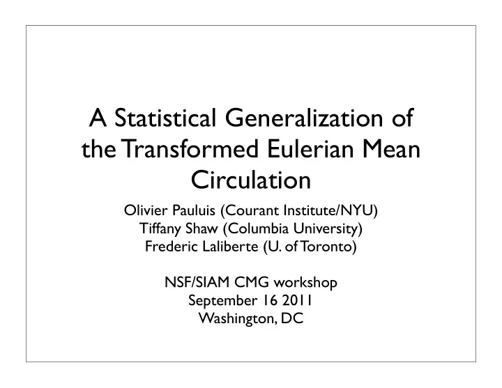
A Statistical Generalization of the Transformed Eulerian Mean Circulation

Olivier Pauluis (Courant Institute/NYU) Tiffany Shaw (Columbia University) Frederic Laliberte (U. of Toronto) NSF/SIAM CMG workshop September 16 2011 Washington, DC

• This requires some averaging, usual both in time and longitude.
• The circulation can be diagnosed by computing the stream

function:

Stream function wind (kg/s) latitude

Ψ(ϕ, p) = 2πv acosϕ

p psurf

∫

dp g

How to describe the circulation?

• Eulerian-mean circulation exhibits the ‘classic’

three-cell structure.

• But the Ferrel cell is a reverse circulation that

transports energy toward the equator.

Ferrel cells Hadley cells Polar cell Polar cell Equator 45S 45N

• BUT the mean meridional circulation depends very

strongly on the vertical coordinate which is used for the averaging.

from Pauluis et al.(2010) ‘dry’ circulation averaged

• n surfaces of constant

potential temperature ‘moist’ circulation averaged

• n surfaces of constant

equivalent potential temperature

Why the circulation in eulerian and isentropic coordinates are in the opposite direction?

• In the midlatitudes, the flow is highly turbulent: the meridional

velocity alternates between poleward and equatorward at all levels.

v > 0 v < 0

longitude

In the stormtracks: Eulerian-mean circulation

• In the midlatitudes, the flow is highly turbulent: the meridional

velocity alternates between poleward and equatorward at all levels.

• This idealized eddies is associated with a poleward flow at

high pressure/low level, and equatorward flow at high level

v > 0 v < 0

Isobaric surface

v p < 0 at low pressure v p > 0 at high pressure

longitude

Thickness variations are such that the upper isentropic layer encompass larger fraction of the poleward flow. Such pattern also corresponds to a net poleward energy mass transport.

Potential temperature surface

v > 0 v < 0

ρθv > 0 at high θ ρθv < 0 at low θ

Warm Cold longitude

In the stormtracks: Isentropic circulation

Dry isentrope

• Moist isentropes found in the upper troposphere

also intersects the Earth’s surface.

• Such situation corresponds to a poleward flow
• f warm, moist air near the surface.

Moist isentrope longitude

v > 0 v < 0

Moist air moving poleward

In the stormtracks: Circulation on moist isentropes

• The global circulation has two poleward

components in the midlatitudes:

– an upper tropospheric branch of high θe-θl; – an a lower branch of warm, most air with high θe- low θl, which ascent into the upper troposphere within the stormtracks.

• Mass transport is comparable in each branch.

Circulation on dry isentropes ‘Moist’ branch: additional mass flow on moist isentropes

• The streamfunction in an arbitrary

coordinate can be defined as

• It is straightforward to compute given 4

dimensional data.

• How to recover it if we are only given the

time mean circulation and eddy statistics?

?

Transformed Eulerian Mean (TEM) Circulation

Text

ζ (p)

TEM residual circulation: Eulerian-mean circulation Eddy component

Transformed Eulerian Mean (TEM) Circulation

Text

ζ (p)

TEM residual circulation: Eulerian-mean circulation Eddy component Great, but TEM breaks down when is not stratified

ζ (p)

The Statistical Transformed Eulerian Mean (STEM) Circulation

We introduce a join distribution of the meridional mass transport so that the streamfunction can be written as We assume that at each pressure and latitude, the velocity and obey a Gaussian distribution with the covariance matrix

Under these assumptions, the mean velocity for a given value of is The join distribution follows: with

potential temperature latitude ,mean DJF −80 −60 −40 −20 20 40 60 80 260 280 300 320 340 360 potential temperature latitude ,eddy DJF −80 −60 −40 −20 20 40 60 80 260 280 300 320 340 360 potential temperature latitude ,STEM DJF −80 −60 −40 −20 20 40 60 80 260 280 300 320 340 360 potential temperature latitude DJF −80 −60 −40 −20 20 40 60 80 260 280 300 320 340 360

• equiv. potential temperature

latitude

• e,mean DJF

−80 −60 −40 −20 20 40 60 80 260 280 300 320 340 360

• equiv. potential temperature

latitude

• e,eddy DJF

−80 −60 −40 −20 20 40 60 80 260 280 300 320 340 360

• equiv. potential temperature

latitude

• e,STEM DJF

−80 −60 −40 −20 20 40 60 80 260 280 300 320 340 360

• equiv. potential temperature

latitude

• e

DJF −80 −60 −40 −20 20 40 60 80 260 280 300 320 340 360

• equiv. potential temperature

latitude

• e,eddy,SH DJF

−80 −60 −40 −20 20 40 60 80 260 280 300 320 340 360

• equiv. potential temperature

latitude

• e,eddy,LH DJF

−80 −60 −40 −20 20 40 60 80 260 280 300 320 340 360

• equiv. potential temperature
• e,eddy,SH JJA

− − − − 340 360

• equiv. potential temperature
• e,eddy,LH JJA

− − − − 340 360

• equiv. potential temperature

latitude

• e,eddy,SH DJF

−80 −60 −40 −20 20 40 60 80 260 280 300 320 340 360

• equiv. potential temperature

latitude

• e,eddy,LH DJF

−80 −60 −40 −20 20 40 60 80 260 280 300 320 340 360

• equiv. potential temperature
• e,eddy,SH JJA

−80 −60 −40 −20 20 40 60 80 260 280 300 320 340 360

• equiv. potential temperature
• e,eddy,LH JJA

−80 −60 −40 −20 20 40 60 80 260 280 300 320 340 360

Sensible heat contribution peaks in the midlatitudes

• equiv. potential temperature

latitude

• e,eddy,SH DJF

−80 −60 −40 −20 20 40 60 80 260 280 300 320 340 360

• equiv. potential temperature

latitude

• e,eddy,LH DJF

−80 −60 −40 −20 20 40 60 80 260 280 300 320 340 360

• equiv. potential temperature
• e,eddy,SH JJA

−80 −60 −40 −20 20 40 60 80 260 280 300 320 340 360

• equiv. potential temperature
• e,eddy,LH JJA

−80 −60 −40 −20 20 40 60 80 260 280 300 320 340 360

Sensible heat contribution peaks in the midlatitudes Latent heat contribution peaks on the equatorward side of the stormtracks

• equiv. potential temperature

latitude

• e,eddy,SH DJF

−80 −60 −40 −20 20 40 60 80 260 280 300 320 340 360

• equiv. potential temperature

latitude

• e,eddy,LH DJF

−80 −60 −40 −20 20 40 60 80 260 280 300 320 340 360

• equiv. potential temperature
• e,eddy,SH JJA

−80 −60 −40 −20 20 40 60 80 260 280 300 320 340 360

• equiv. potential temperature
• e,eddy,LH JJA

−80 −60 −40 −20 20 40 60 80 260 280 300 320 340 360

Sensible heat contribution peaks in the midlatitudes Latent heat contribution peaks on the equatorward side of the stormtracks Latent heat contribution extends far in the tropics

• equiv. potential temperature

latitude

• e,eddy,SH DJF

−80 −60 −40 −20 20 40 60 80 260 280 300 320 340 360

• equiv. potential temperature

latitude

• e,eddy,LH DJF

−80 −60 −40 −20 20 40 60 80 260 280 300 320 340 360

• equiv. potential temperature
• e,eddy,SH JJA

−80 −60 −40 −20 20 40 60 80 260 280 300 320 340 360

• equiv. potential temperature
• e,eddy,LH JJA

−80 −60 −40 −20 20 40 60 80 260 280 300 320 340 360

Sensible heat contribution peaks in the midlatitudes Latent heat contribution peaks on the equatorward side of the stormtracks Latent heat contribution extends far in the tropics Both contributions overlap across the stormtracks, so that the total circulation is larger than either component.

Relationship between TEM and STEM

• It can be shown formally that as the variance

goes to 0, the STEM streamfunction converges toward the TEM, i.e:

potential temperature latitude ,STEM DJF variance = 64 K2 −80 −60 −40 −20 20 40 60 80 260 280 300 320 340 360 potential temperature latitude ,STEM DJF variance = 16 K2 −80 −60 −40 −20 20 40 60 80 260 280 300 320 340 360 potential temperature latitude ,STEM DJF variance = 4 K2 −80 −60 −40 −20 20 40 60 80 260 280 300 320 340 360 potential temperature latitude ,STEM DJF variance = 1 K2 −80 −60 −40 −20 20 40 60 80 260 280 300 320 340 360

Conclusions

• The ‘mean’ atmospheric circulation is highly

sensitive to the averaging method.

• The STEM circulation extends the TEM

circulation to an arbitrary coordinate system by taking advantage of additional eddy statistics.

• The TEM circulation corresponds to the small

variance limit of the STEM circulation.

• The need for new mathematical ideas in geoscience includes the

development of new conceptual and theoretical framework.

• Water vapor and clouds remain a central problem in atmospheric/

climate sciences.

• Statistical and stochastic approaches could be potentially very

useful in atmospheric and oceanic science (for parameterization, data assimilation and parameter estimation).

• Progress is often serendipitous: it hard to predict which

mathematical tool will solve a given physical problems. Active collaborations are keys to sustain successful exchange of ideas.

Some thoughts on CMG: