A Least Angle Regression Control Chart for Multidimensional Data G - - PowerPoint PPT Presentation

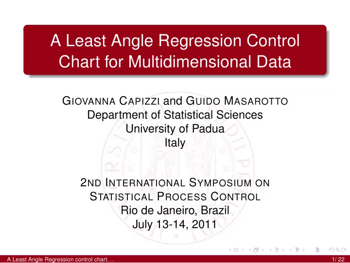
A Least Angle Regression Control Chart for Multidimensional Data

GIOVANNA CAPIZZI and GUIDO MASAROTTO Department of Statistical Sciences University of Padua Italy 2ND INTERNATIONAL SYMPOSIUM ON STATISTICAL PROCESS CONTROL Rio de Janeiro, Brazil July 13-14, 2011

A Least Angle Regression control chart. . . 1/ 22

Outline

1

Multivariate Statistical Monitoring

2

Variable-selection Methods in SPC

3

Proposed Procedure

Reference Model Least Angle Regression Algorithm LAR-EWMA control chart

4

Simulation Results

5

Concluding Remarks and Future Research

A Least Angle Regression control chart. . . 2/ 22

Synopsis

Framework: Phase II monitoring of a normal multivariate vector of product variables. Fault type: Persistent change in the process mean and/or increase in the total dispersion. Problem: Simultaneous monitoring of several variables: how many and which variables are really changed? Proposal: Combination of a variable-selection method (Least Angle Regression) with a multivariate control chart (multivariate EWMA). Results: The LAR-based EWMA is a very competitive statistical tool for handling several change- point scenarios in the high-dimensional framework.

A Least Angle Regression control chart. . . 3/ 22

Multivariate Statistical Monitoring

Possible Frameworks

UNSTRUCTURED:

multivariate vector of quality characteristics

STRUCTURED:

analytical models describing process quality

1

linear and non linear profiles

2

multistage processes

A Least Angle Regression control chart. . . 4/ 22

Multivariate Statistical Monitoring

Possible Approaches

Monitoring the stability of the whole set of product variables (low sensitivity in a high-dimensional context) Monitoring a reduced set of out-of-control product variables. But the shifted components are obviously unknown!

A Least Angle Regression control chart. . . 5/ 22

Variable-selection Methods in SPC

State of the art

Promising approach: combine a suitable variable selection method with the multivariate statistical monitoring Forward search algorithm with a Shewhart-type control chart (Wang and Jiang, 2009) for handling mean changes in the unstructured scenario. LASSO algorithm with a multivariate EWMA, for detecting

1

mean changes in the unstructured case (Zou and Qiu, 2009)

2

changes in multivariate linear profiles (Zou et al. 2010)

A Least Angle Regression control chart. . . 6/ 22

Variable-selection Methods in SPC

Our proposal

LEAST ANGLE REGRESSION WITH A MULTIVARIATE EWMA

1

general model formulation unifying the unstructured and structured framework

2

use of a variable selection method yet unexplored in the SPC framework

3

competitive procedure for detecting changes in process mean and total dispersion for a wide variety

• f change point-scenarios

4

relatively simple tool for fault identification

A Least Angle Regression control chart. . . 7/ 22

Reference Model

Characterization of mean and variance changes

CHANGE-POINT MODEL

yt ∼ Nn(µ µ µ,Σ Σ Σ) if t < τ (in-control) Nn(µ µ µ +δ δ δ,Ω Ω Ω) if t ≥ τ (out-of-control)

MEAN SHIFT

δ δ δ = Fβ β β

F n×p: matrix of known constants; β β β p×1: vector of unknown parameters . DISPERSION INCREASE

EOC[ξ 2

t ] > n ⇐ Ω

Ω Ω−Σ Σ Σ positive definite matrix

with ξ 2

t = (yt − µ

µ µ)Σ Σ Σ−1(yt − µ µ µ)′ .

A Least Angle Regression control chart. . . 8/ 22

Reference Model

Frameworks and characterization of δ δ δ

UNSTRUCTURED

[δi] = [βi] ⇐ ⇒ F = In

PROFILE

[δi] = [g(xi)] = p

∑

j=1

βjfj(xi)

• e.g. δi = β1 +β2xi +β3x2

i for i = 1,...,n.

MULTISTAGE PROCESS

Standard state space representations of a process with n stages can be written in the desired form. yt,i = µi +cixt,i +vt,i xt,i = dixt,i−1 +βiI{t≥τ} +wt,i (i = 1,...,n)

A Least Angle Regression control chart. . . 9/ 22

Reference Model

Monitoring stability ← → Testing hypotheses on β β β

Multivariate EWMA control statistic zt = (1−λ)zt−1 +λ(yt − µ µ µ) with z0 = 0n, 0 < λ ≤ 1. Linear model zt = Fβ β β +at, with at ∼ Nn (0n,λ/(1−λ)Σ Σ Σ)

MONITORING STABILITY OF PROCESS MEAN

H0 = {the process is in control} ⇐ ⇒ {β β β = 0} H1 = {the process is out of control} ⇐ ⇒ {How many βj are non zero? One, two....all? }

A Least Angle Regression control chart. . . 10/ 22

Least Angle Regression algorithm

Main steps

1

Start with all the p coefficients equal to zero.

2

Build up estimates of the unknown mean in successive steps: each step adding one variable.

3

Reach the full least square solution in p steps (using all the variables).

STEP k

{j1,...,jk}

• variables selected by LAR

⇐ ⇒ {βj1,...,βjk}

• just k parameters are assumed = 0

A Least Angle Regression control chart. . . 11/ 22

LAR-EWMA control chart

Hypotheses systems and control statistics

MEAN CHANGE

HYPOTHESIS CONTROL STATISTIC . βj1 = 0,...,βjk = 0, βjk+1 = ··· = βjp = 0 Likelihood ratio test: St,k (k = 1,...,p)

VARIATION INCREASE

HYPOTHESIS CONTROL STATISTIC β β β = 0p and E[ξ 2

t ] > n

St,p+1 = x max

• 1,(1−λ)St−1,p+1 +λ ξ 2

t

n

• with S0,p+1 = 1

A Least Angle Regression control chart. . . 12/ 22

LAR-EWMA control chart

Control statistic, stopping rule, fault identification

Control statistic Wt = max

k=1,...,p+1

St,k −ak bk Alarm time t⋆ = min{t : Wt > h} Fault Identification k⋆ = min

• k : St⋆,k −ak

bk > h

• k⋆ ≤ p : {plausible mean shift}

k⋆ = p +1 : {plausible dispersion increase}

A Least Angle Regression control chart. . . 13/ 22

LAR-EWMA control chart

Control chart design

SMOOTHING CONSTANT λ (0.1, 0.3) normal distribution (0.03, 0.05) skewed and heavy-tailed distributions CONTROL LIMIT h h is determined to obtain a desired value of the in-control ARL via simulation, using the Polyak-Ruppert stochastic approximation algorithm.

A Least Angle Regression control chart. . . 14/ 22

Simulation Results

Competitive control charts

MEAN CHANGE AND NO VARIANCE CHANGE UNSTRUCTURED SCENARIO MULTISTAGE PROCESSES REWMA (Hawkins, 1991,1993) MEWMA (Lowry et al.,1992) MEWMA (Lowry et al.,1992) DEWMA (Zou and Tsung, 2008) LEWMA (Zou and Qiu, 2009) MEAN CHANGE AND VARIANCE INCREASE PARAMETRIC PROFILE NONPARAMETRIC PROFILE KMW (Kim, et al. 2003)) NEWMA (Zou et al., 2008) PEWMA (Zou et al.,2007)

A Least Angle Regression control chart. . . 15/ 22

Simulation Results

Investigation of a wide variety of out-of-control scenarios (unstructured and structured)

1

large range of size shifts

2

different combinations of shifted components or locations: one, more than one.

3

mean shifts and/or variance increases

performance measure: Average Run Length summary performance measure: the Relative Mean Index (Han and Tsung, 2006). Very small RMI values = ⇒ best or close to the best chart.

A Least Angle Regression control chart. . . 16/ 22

Simulation Results

The Relative Mean Index (Han and Tsung, 2006)

The RMI is a summary performance measure defined as RMI = 1 N

N

∑

l=1

RMIl = 1 N

N

∑

l=1

ARLδ

δ δ l −MARLδ δ δ l

MARLδ

δ δ l

1

N total number of shifts

2

ARLδ

δ δ l out-of-control ARL for detecting δ

δ δ l

3

MARLδ

δ δ l smallest out-of-control ARL, among the

compared charts, for detecting δ δ δ l

4

RMIl relative efficiency of a chart in detecting δ δ δ l compared to the best chart.

A Least Angle Regression control chart. . . 17/ 22

Linear Profile

IC: yt,i ∼ N(0,1). OC: yt,i ∼ N(β1 +β2xi,ω2), i = 1,...,4, xi = −1,−1/3,1/3,1

Shifts PEWMA KMW LAR-EWMA β1 = 0.1 293.08 296.40 272.39 β1 = 0.3 46.16 43.04 39.55 β1 = 1 4.65 4.29 4.22 β2 = 0.2 180.73 182.79 163.19 β2 = 0.4 46.84 43.66 40.14 β2 = 1.2 5.41 4.99 4.90 β1 = 0.1, β2 = 0.1 230.79 243.60 215.11 β1=0.4,β2 = 0.2 20.69 21.14 18.80 β1 = 0.4 , β2 = 0.6 10.39 12.34 10.05 β1 = 0.6, β2 = 0.6 7.11 8.16 6.88 β1 = 0.1, ω = 1.2 45.88 50.95 38.78 β1 = 0.3, ω = 1.2 21.55 23.77 20.14 β1 = 1, ω = 1.2 4.44 4.29 4.08 β2 = 0.2, ω = 1.2 38.68 43.46 33.71 β2 = 0.4, ω = 1.2 21.80 23.93 20.13 β2 = 1.2, ω = 1.2 5.12 4.97 4.72 β1 = 0.1, β2 = 0.1, ω = 1.2 42.47 47.36 36.26 β1 = 0.4, β2 = 0.2, ω = 1.2 13.74 15.14 13.02 β1 = 0.4, β2 = 0.6, ω = 1.2 8.60 9.96 8.36 β1 = 0.6, β2 = 0.6, ω = 1.2 6.41 7.29 6.19 ω = 1.2 53.39 58.17 43.24 ω = 1.5 11.06 12.35 7.90 ω = 2 4.37 4.71 3.03 RMI 0.13 0.19 0.00 A Least Angle Regression control chart. . . 18/ 22

Simulation Results: RMI

ARL0 = 500, λ = 0.2, τ = 1

“Unstructured” LAR-EWMA MEWMA REWMA LEWMA n = 15 0.02 0.24 0.32 0.10 Linear Profile LAR-EWMA PEWMA KMW n = 4 0.00 0.13 0.19 n = 10 0.01 0.07 0.11 Cubic Profile LAR-EWMA PEWMA KMW n = 8 0.00 0.24 0.36 n = 15 0.00 0.23 0.31 Non-parametric profile LAR-EWMA NEWMA n = 20 0.05 0.28 n = 40 0.06 0.30 Multistage process LAR-EWMA MEWMA DEWMA n = 20;ci = di = 1 0.02 0.24 0.10 n = 20;ci = 1.2;di = 0.8 0.06 0.22 0.18

A Least Angle Regression control chart. . . 19/ 22

Concluding Remarks and Future Research

Advantages and Novel Aspects

The LAR-based multivariate EWMA

• ffers an unifying approach for handling the

multivariate statistical monitoring in both the unstructured and structured framework

Flexible choices of F in a quite general model formulation

makes use of a relatively easier and faster variable selection method shows some appealing enhancements:

a control statistic for detecting increases in total dispersion a simple tool for fault detection.

A Least Angle Regression control chart. . . 20/ 22

Concluding remarks and future research

Future Research

A more general formulation for dispersion changes. Generalization of the LAR algorithm for non-normal data (but how is possible to handle dispersion changes in a distribution-free way?) Design of variable sampling interval version of the LAR-EWMA.

A Least Angle Regression control chart. . . 21/ 22

THANKS...

SINCE 1222

“UNIVERSA UNIVERSIS PATAVINA LIBERTAS”

(Paduan Freedom is Complete and for Everyone) Anatomy Theatre (1594) Galileo Galilei’s desk (≈1605)

A Least Angle Regression control chart. . . 22/ 22