A hybrid metaheuristic for production planning Jo ao Pedro PEDROSO - PowerPoint PPT Presentation
A hybrid metaheuristic for production planning Jo ao Pedro PEDROSO Universidade do Porto, Portugal jpp@ncc.up.pt Makoto OHNISHI Fujitsu Research Institute, Japan ohnishi@fri.fujitsu.com Mikio KUBO Tokyo University of Marine Science and
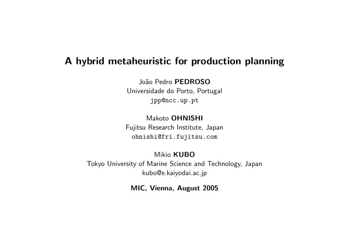
A hybrid metaheuristic for production planning Jo˜ ao Pedro PEDROSO Universidade do Porto, Portugal jpp@ncc.up.pt Makoto OHNISHI Fujitsu Research Institute, Japan ohnishi@fri.fujitsu.com Mikio KUBO Tokyo University of Marine Science and Technology, Japan kubo@e.kaiyodai.ac.jp MIC, Vienna, August 2005
Introduction This work deals with two problems arising in production planning: • lot sizing • scheduling • usually these problems are treated separately • for both problems: exact solution can be rather hard • appropriate solvers are different: – lot sizing − → mixed integer programming (MIP) – scheduling − → constraint programming • metaheuristics: provide a unified framework • this work: focus on the integration 1
Motivation • Practical problem: – large industry – stable demand – production site where raw materials are transformed into end products. • Currently: – scheduling operations come from customer orders – scheduling based on feasibility: no notion of cost involved – demand is stable − → why not think about lot sizes? • Aim: – formalise the problem – lot sizing + scheduling − → scheduling operations derived from good/optimal lot sizes – implement a prototype – check feasibility of the approach with nearly-real data • Planning: – Short term (scheduling): monthly basis – Medium term (lot sizing): yearly basis 2
Background Previous work in this area: LISCOS European project • Exact approaches • MIP for lot sizing • Constraint programming for scheduling • Both are commercial solvers • Cost − → not appropriate for prototyping − → metaheuristics 3
Lot sizing Considering all the orders, for the whole of Demand the planning horizon, decide: Lot • quantity of each lot to be produced • when to produce each lot • (not concerned with order of production in the machines) Machine Machine Machine t=1 1 2 3 Machine Machine Machine t=2 1 2 3 . . . 4
Scheduling For each operation of a given period of the Operations lot sizing problem: • assign it to a machine • assign it an order in the operations of that machine • detail: machines can operate in several modes : – full capacity − → higher cost – reduced capacity − → lower cost Machine Machine Machine 1 2 3 5
Time horizons • are different for lot sizing and for scheduling • horizon for scheduling ↔ one period of lot sizing model • usually: scheduling only for the first period of lot sizing lot sizing 1 2 3 4 5 6 7 8 9 10 11 12 1 2 3 4 5 6 7 8 9 10 11 12 13 14 15 scheduling 6
Main solution procedure Start Solve lot Prepare sizing prob scheduling problem Solve Add constraint scheduling cutting current problem solution N Y Feasible? Stop 7
Lot sizing model • Costs: – setup (fixed) costs – variable production costs – inventory – backlog • Decision varibles: – manufacture or not of a product in each period: setup, binary variable y pmt ∗ y pmt = 1 if product p is manufactured in machine m during period t ∗ y pmt = 0 otherwise – amount produced: continuous variable x pmt ∗ corresponding to y pmt . ∗ x pmt > 0 ⇒ y pmt = 1 – inventory h pt and backlog g pt 8
Objective setup costs: F = P P P t ∈T f pmt y pmt p ∈P m ∈M • f pmt is the cost of setting up machine m on period t for producing p variable costs: V = P P P t ∈T v pmt x pmt p ∈P m ∈M • v pmt is the variable cost of production of p on machine m , period t inventory costs: I = P P t ∈T i pt h pt p ∈P • h pt is the amount of product p that is kept in inventory at the end of period t • i pt is the unit inventory cost for product p on period t backlog costs: B = P P t ∈T b pt g pt p ∈P • g pt is the amount of product p that failed to meet demand at the end of period t • b pt is the unit backlog cost for product p on period t . objective: minimise z = F + V + I + B 9
Constraints: flow conservation: X h p,t − 1 − g p,t − 1 + x pmt = D pt + h pt − g pt ∀ p ∈ P , ∀ t ∈ T . m ∈M p h p 0 , h pT : initial and final inventory g p 0 , g pT : initial and final backlog time availability on each period: „ x pmt « X + τ pmt y pmt ≤ A mt ∀ m ∈ M , ∀ t ∈ T . γ pm p ∈P : m ∈M p γ pm is the total capacity of production of product p on machine m per time unit τ pmt is the setup time required if there is production of p on machine m during period t A mt is the number of time units available for production on machine m during period t . setup constraints: x pmt ≤ γ pm A mt y pmt 10
minimise z = F + V + I + B X X X subject to : F = f pmt y pmt p ∈P m ∈M t ∈T X X X V = v pmt x pmt p ∈P m ∈M t ∈T X X I = i pt h pt p ∈P t ∈T X X B = b pt g pt p ∈P t ∈T X h p,t − 1 − g p,t − 1 + x pmt = D pt + h pt − g pt , ∀ p ∈ P , ∀ t ∈ T m ∈M p „ x pmt « X + τ pmt y pmt ≤ A mt , ∀ m ∈ M , ∀ t ∈ T γ pm p ∈P : m ∈M p ∀ p ∈ P , ∀ m ∈ M p , ∀ t ∈ T x pmt ≤ γ pm A mt y pmt R + F, V, I, B ∈ I R + , h pt , g pt ∈ I ∀ p ∈ P , ∀ t ∈ T R + , y pmt ∈ { 0 , 1 } , x pmt ∈ I ∀ p ∈ P , ∀ m ∈ M , ∀ t ∈ T 11
Construction: relax-and-fix-one-product • construction of a solution: based on partial relaxations of the initial problem • variant of the classic relax-and-fix heuristic 12
Relax-and-fix • each period is treated independently t=1 • relax all the variables except those of period 1 : – keep y pm 1 integer – relax integrity for all other y pmt t=2 • solve this MIP, determining heuristic values for ¯ y pm 1 . . . t=T 13
Relax-and-fix • each period is treated independently t=1 • relax all the variables except those of period 1 : – keep y pm 1 integer – relax integrity for all other y pmt t=2 • solve this MIP, determining heuristic values for ¯ y pm 1 • move to the second period: . . . – variables of the first period are fixed at y pm 1 = ¯ y pm 1 – variables y pm 2 are integer t=T – and all the other y pmt relaxed • this determines the heuristic value for y pm 2 14
Relax-and-fix • each period is treated independently t=1 • relax all the variables except those of period 1 : – keep y pm 1 integer – relax integrity for all other y pmt t=2 • solve this MIP, determining heuristic values for ¯ y pm 1 • move to the second period: . . . – variables of the first period are fixed at y pm 1 = ¯ y pm 1 – variables y pm 2 are integer – and all the other y pmt relaxed t=T • this determines the heuristic value for y pm 2 • these steps are repeated, until all the y variables are fixed 15
Relax-and-fix • each period is treated independently t=1 • relax all the variables except those of period 1 : – keep y pm 1 integer – relax integrity for all other y pmt t=2 • solve this MIP, determining heuristic values for ¯ y pm 1 • move to the second period: . . . – variables of the first period are fixed at y pm 1 = ¯ y pm 1 – variables y pm 2 are integer – and all the other y pmt relaxed t=T • this determines the heuristic value for y pm 2 • these steps are repeated, until all the y variables are fixed 16
Relax-and-fix heuristic. • reported to provide very good solutions for many lot sizing problems • however, for large instances the exact MIP solution of even a single period can be too time consuming • we propose a variant were each MIP determines only the variables of one period that concern a single product → relax-and-fix-one-product 17
Relax-and-fix-one-product variant. RelaxAndFixOneProduct () t=1 (1) relax all y pmt as continuous variables (2) for t = 1 to T (3) foreach p ∈ P t=2 foreach m ∈ M p (4) (5) set y pmt as integer y pmt , ∀ m ∈ M p (6) solve MIP → ¯ . . . foreach m ∈ M p (7) (8) fix y pmt := ¯ y pmt (9) return ¯ y t=T 18
Relax-and-fix-one-product variant. RelaxAndFixOneProduct () t=1 (1) relax all y pmt as continuous variables (2) for t = 1 to T (3) foreach p ∈ P t=2 foreach m ∈ M p (4) (5) set y pmt as integer y pmt , ∀ m ∈ M p (6) solve MIP → ¯ . . . foreach m ∈ M p (7) (8) fix y pmt := ¯ y pmt (9) return ¯ y t=T 19
Relax-and-fix-one-product variant. RelaxAndFixOneProduct () t=1 (1) relax all y pmt as continuous variables (2) for t = 1 to T (3) foreach p ∈ P t=2 foreach m ∈ M p (4) (5) set y pmt as integer y pmt , ∀ m ∈ M p (6) solve MIP → ¯ . . . foreach m ∈ M p (7) (8) fix y pmt := ¯ y pmt (9) return ¯ y t=T 20
Relax-and-fix-one-product variant. RelaxAndFixOneProduct () t=1 (1) relax all y pmt as continuous variables (2) for t = 1 to T (3) foreach p ∈ P t=2 foreach m ∈ M p (4) (5) set y pmt as integer y pmt , ∀ m ∈ M p (6) solve MIP → ¯ . . . foreach m ∈ M p (7) (8) fix y pmt := ¯ y pmt (9) return ¯ y t=T 21
Relax-and-fix-one-product variant. RelaxAndFixOneProduct () t=1 (1) relax all y pmt as continuous variables (2) for t = 1 to T (3) foreach p ∈ P t=2 foreach m ∈ M p (4) (5) set y pmt as integer y pmt , ∀ m ∈ M p (6) solve MIP → ¯ . . . foreach m ∈ M p (7) (8) fix y pmt := ¯ y pmt (9) return ¯ y t=T 22
Relax-and-fix-one-product variant. RelaxAndFixOneProduct () t=1 (1) relax all y pmt as continuous variables (2) for t = 1 to T (3) foreach p ∈ P t=2 foreach m ∈ M p (4) (5) set y pmt as integer y pmt , ∀ m ∈ M p (6) solve MIP → ¯ . . . foreach m ∈ M p (7) (8) fix y pmt := ¯ y pmt (9) return ¯ y t=T 23
Recommend
More recommend
Explore More Topics
Stay informed with curated content and fresh updates.

