[PPT] - A Hierarchy of System Specification Basis of System Specification PowerPoint Presentation

SLIDE 1

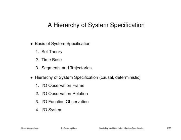
A Hierarchy of System Specification

Basis of System Specification
1. Set Theory
2. Time Base
3. Segments and Trajectories
Hierarchy of System Specification (causal, deterministic)
1. I/O Observation Frame
2. I/O Observation Relation
3. I/O Function Observation
4. I/O System

Hans Vangheluwe hv@cs.mcgill.ca Modelling and Simulation: System Specification 1/58

SLIDE 2

5. Multicomponent Specifications

– Modular – Non-modular

Non-causal models

Hans Vangheluwe hv@cs.mcgill.ca Modelling and Simulation: System Specification 2/58

SLIDE 3

System Specification

Start from observations of structure and behaviour
Build progressively more complex/detailed models
Use models to answer questions about structure and behaviour
OO terminology: model composed of

– objects, with attributes

✁

indicative or relational

✁

have type (set of possible values)

– relationships between objects

Hans Vangheluwe hv@cs.mcgill.ca Modelling and Simulation: System Specification 3/58

SLIDE 4

Set Theory for Abstraction

✂

1

✄

2

✄✆☎ ☎ ☎ ✄

9

✝ ✂

a

✄

b

✄✆☎ ☎ ☎ ✄

z

✝ ✞ ✄ ✞✠✟ ✄ ✞ ✟

∞

✡ ✄ ✡ ✟ ✄ ✡ ✟

∞

EV

☛ ✂

ARRIVAL

✄

DEPARTURE

✝

EV φ

☛

EV

☞ ✂

φ

✝

A

✌

B

☛ ✂ ✍

a

✄

b

✎ ✏

a

✑

A

✄

b

✑

B

✝

Hans Vangheluwe hv@cs.mcgill.ca Modelling and Simulation: System Specification 4/58

SLIDE 5

Relationships over Sets

1. Nominal Scale
2. Ordinal Scale
3. Interval Scale
4. Ratio Scale

Hans Vangheluwe hv@cs.mcgill.ca Modelling and Simulation: System Specification 5/58

SLIDE 6

Nominal Scale Symbols are used to label or classify data

A scale that assigns a category label to an individual. For example, eye color is a categorical scale. Establishes no explicit ordering on the category labels. Categorical scales are also called discrete or symbolic scales, or nominal scales when the label (e.g., “green”) is a name. Only a notion of equivalence “

☛

” is defined with properties:

1. Reflexivity: x

☛

x

✒

x

✓ ☛

x.

2. Symmetry of equivalence: x

☛

y

✔

y

☛

x.

3. Transitivity: x

☛

y

✕

y

☛

z

✖

x

☛

z.

Hans Vangheluwe hv@cs.mcgill.ca Modelling and Simulation: System Specification 6/58

SLIDE 7

Ordinal Scale

A scale in which data can be ranked, but in which no arithmetic transformations are meaningful. For example, wind speed

✑ ✂

high, medium, low

✝

. We would not say that the difference between high and medium wind speed is equal to (or any arithmetic transformation of) the difference between a medium and low wind speed. The distances between points on an ordinal scale are not meaningful. In addition to a notion of equivalence, a notion of order

✗

is defined with properties:

1. Symmetry of equivalence: x

☛

y

✔

y

☛

x.

2. Asymmetry of order: x

✗

y

✖

y

✓ ✗

x.

3. Irreflexivity: x

✓ ✗

x.

4. Transitivity: x

✗

y

✕

y

✗

z

✖

x

✗

z.

Hans Vangheluwe hv@cs.mcgill.ca Modelling and Simulation: System Specification 7/58

SLIDE 8

Partial ordering

The ordering may be partial (some data items cannot be compared). Used to model uncertainty, multiplicity, concurrency, . . . .

t1 t2 t3 t4 t5 t6 t7

The ordering may be total (all data items can be compared).

✘

x

✄

y

✑

X : x

✗

y

✒

y

✗

x

✒

x

☛

y

Hans Vangheluwe hv@cs.mcgill.ca Modelling and Simulation: System Specification 8/58

SLIDE 9

Interval Scale

A scale where distances between data are meaningful. On interval measurement scales, one unit on the scale represents the same magnitude on the characteristic being measured across the whole range

f the scale. Interval scales do not have a “true” zero point, however, and

therefore it is not possible to make statements about how many times higher one value is than another. An example is the Celcius scale for temperature. Equal differences on this scale represent equal differences in temperature, but a temperature of 30 degrees is not twice as warm as one of 15 degrees. In addition to equivalence and order, a notion of interval is defined. The choice of a zero point is arbitrary.

Hans Vangheluwe hv@cs.mcgill.ca Modelling and Simulation: System Specification 9/58

SLIDE 10

Ratio Scale

A scale in which both intervals between values and ratios of values are

meaningful. For example, temperature measured in degrees Kelvin is a

ratio scale because we know a meaningful zero point (absolute zero). A temperature of 300K is twice as warm as 150K. Compare this to interval scales in which ratios are not meaningful and

rdinal scales in which intervals are not meaningful.

Hans Vangheluwe hv@cs.mcgill.ca Modelling and Simulation: System Specification 10/58

SLIDE 11

Time Base

time

☛ ✙

T

✄ ✗ ✚

Dynamic system: irreversible passage of time.
Set T, ordering relation

✗

n elements of T.

– transitive: A

✗

B

✕

B

✗

C

✛

A

✗

C – irreflexive: A

✓ ✗

A – antisymmetric: A

✗

B

✛

B

✓ ✗

A

Ordering:

– Total (linear) ordering

✘

t

✄

t

✜ ✑

T : t

✗

t

✜ ✒

t

✜ ✗

t

✒

t

☛

t

✜

– Partial ordering: uncertainty, multiplicity, concurrency, . . . .

Hans Vangheluwe hv@cs.mcgill.ca Modelling and Simulation: System Specification 11/58

SLIDE 12

Past, Future, Intervals

Past: Tt

✢ ☛ ✂

τ

✏

τ

✑

T

✄

τ

✗

t

✝

Future: T

✣

t

☛ ✂

τ

✏

τ

✑

T

✄

t

✗

τ

✝

✙

t means

✤

t or

✥

t

Interval T

✦

tb

✧

te

★

Abelian group

✍

T

✄✪✩ ✎

with zero 0 and inverse

✫

t

Order preserving

✩

: t1

✗

t2

✛

t1

✩

t

✗

t2

✩

t

Lower bound, upper bound
Time bases:

✂

NOW

✝

,

✡

: continuous,

✞

r isomorphic: discrete,

partial ordering.

Hans Vangheluwe hv@cs.mcgill.ca Modelling and Simulation: System Specification 12/58

SLIDE 13

Time Bases for hybrid system models

TD TC (tc, td)

Hans Vangheluwe hv@cs.mcgill.ca Modelling and Simulation: System Specification 13/58

SLIDE 14

Behaviour over Time: Segments and Trajectories

With time base, describe behaviour over time
Time function, trajectory, signal: f : T

✖

A

Restriction to T

✜ ✬

T f

✏

T

✜

: T

✜ ✖

A,

✘

t

✑

T

✜

: f

✏

T

✜ ✍

t

✎ ☛

f

✍

t

✎

– Past of f : f

✏

Tt

★

– Future of f : f

✏

T

✦

t

Restriction to an interval: segment

✭

behaviour ω :

✙

t1

✄

t2

✚ ✖

A

Ω

☛ ✍

A

✄

T

✎

set of all segments

Hans Vangheluwe hv@cs.mcgill.ca Modelling and Simulation: System Specification 14/58

SLIDE 15

Segments

Length l : Ω

✖

T

✟

Contiguous segments if domains are contiguous

✙

t1

✄

t2

✚ ✄ ✙

t3

✄

t4

✚ ✄

t2

☛

t3

Concatenation of contiguous segments: ω1
ω2

ω1

ω2

✍

t

✎ ☛

ω1

✍

t

✎ ✄ ✘

t

✑

dom

✍

ω1

✎

ω1

ω2

✍

t

✎ ☛

ω2

✍

t

✎ ✄ ✘

t

✑

dom

✍

ω2

✎

Must remain function: unique values !
Ω closed under concatenation
Left and right segments:

ωt

★

ω

✦

t

☛

ω

Hans Vangheluwe hv@cs.mcgill.ca Modelling and Simulation: System Specification 15/58

SLIDE 16

Types of Segments

Continuous: ω :

✙

t1

✄

t2

✚ ✖ ✡

n

Piecewise continuous
Piecewise constant
Event segments: ω :

✙

t1

✄

t2

✚ ✖

A

☞ ✂

φ

✝

Correspondence between

piecewise constant and event segments (later, state trajectory)

Hans Vangheluwe hv@cs.mcgill.ca Modelling and Simulation: System Specification 16/58

SLIDE 17

Types of Segments

T T T T continuous piecewise continuous piecewise constant discrete event

Hans Vangheluwe hv@cs.mcgill.ca Modelling and Simulation: System Specification 17/58

SLIDE 18

Cashier-Queue System

Physical View Queue Cashier Departure Arrival Departure Queue Abstract View Cashier [ST distribution] [IAT distribution] Arrival

Hans Vangheluwe hv@cs.mcgill.ca Modelling and Simulation: System Specification 18/58

SLIDE 19

Trajectories

state= queue_length x cashier_state

queue_length T 1 2 10 20 30 40 50 cashier_state Busy Idle T 10 20 30 40 50 T Input Events Arrival 10 20 30 40 50

E1 E2

T Output Events Departure 10 20 30 40 50

E3 E4

Hans Vangheluwe hv@cs.mcgill.ca Modelling and Simulation: System Specification 19/58

SLIDE 20

I/O Observation Frame

O

☛ ✙

T

✄

X

✄

Y

✚

T is time-base:

✞

(discrete-time),

✡

(continuous-time)

X input value set:

✡

n

✄

EV φ

Y output value set: system response

Hans Vangheluwe hv@cs.mcgill.ca Modelling and Simulation: System Specification 20/58

SLIDE 21

I/O Relation Observation

IORO

☛ ✙

T

✄

X

✄

Ω

✄

Y

✄

R

✚

✙

T

✄

X

✄

Y

✚

is Observation Frame

Ω is the set of all possible input segments
R is the I/O relation

Ω

✬ ✍

X

✄

T

✎

, R

✬

Ω

✌ ✍

Y

✄

T

✎ ✍

ω

✄

ρ

✎ ✑

R

✛

dom

✍

ω

✎ ☛

dom

✍

ρ

✎

ω :

✙

ti

✄

t f

✚ ✖

X: input segment

ρ :

✙

ti

✄

t f

✚ ✖

Y: output segment

note: not really necessary to observe over same time domain

Hans Vangheluwe hv@cs.mcgill.ca Modelling and Simulation: System Specification 21/58

SLIDE 22

I/O Function Observation

IOFO

☛ ✙

T

✄

X

✄

Ω

✄

Y

✄

F

✚

✙

T

✄

X

✄

Ω

✄

Y

✄

R

✚

is a Relation Observation

Ω is the set of all possible input segments
F is the set of I/O functions

f

✑

F

✛

f

✮

Ω

✌ ✍

Y

✄

T

✎

, where

f is a function such that dom

✍

f

✍

ω

✎ ✎ ☛

dom

✍

ω

✎

f = initial state: unique response to ω
R

☛ ✯

f

✰

F f

Hans Vangheluwe hv@cs.mcgill.ca Modelling and Simulation: System Specification 22/58

SLIDE 23

I/O System

From Descriptive Variables to State.
State summarizes the past of the system.
Future is uniquely determined by

– current state – future input

Hans Vangheluwe hv@cs.mcgill.ca Modelling and Simulation: System Specification 23/58

SLIDE 24

SYS

☛ ✙

T

✄

X

✄

Ω

✄

Q

✄

δ

✄

Y

✄

λ

✚

T

time base

X

input set

ω : T

✖

X

input segment

Q

state set

δ : Ω

✌

Q

✖

Q

transition function

Y

utput set

λ : Q

✖

Y (or Q

✌

X

✖

Y)

utput function

✘

tx

✑ ✥

ti

✄

t f

✤

: δ

✍

ω

✢

ti

✧

tf

✣ ✄

qi

✎ ☛

δ

✍

ω

✢

tx

✧

tf

✣ ✄

δ

✍

ω

✢

ti

✧

tx

✣ ✄

qi

✎ ✎

Closure requirement: Ω closed under concatenation and left segmentation.

Hans Vangheluwe hv@cs.mcgill.ca Modelling and Simulation: System Specification 24/58

SLIDE 25

Composition Property

t_f t_x t_i

Q X T T ω[t_x, t_f] ω[t_i, t_x] ω[t_i, t_f] δ(t_x -> t_f) δ(t_i -> t_x) δ(t_i -> t_f)

Hans Vangheluwe hv@cs.mcgill.ca Modelling and Simulation: System Specification 25/58

SLIDE 26

System under study: T

✱

h controlled liquid

is_full is_empty heat

ff

cool is_cold is_hot

fill empty closed

Hans Vangheluwe hv@cs.mcgill.ca Modelling and Simulation: System Specification 26/58

SLIDE 27

Detailed (continuous) view, ALG + ODE formalism

Inputs (discontinuous

✲

hybrid model):

✳

Emptying, filling flow rate φ

✳

Rate of adding/removing heat W Parameters:

✳

Temperature of influent Tin

✳

Cross-section surface of vessel A

✳

Specific heat of liquid c

✳

Density of liquid ρ State variables:

✳

Temperature T

✳

Level of liquid l Outputs (sensors):

✳

is low

✴

is high

✴

is cold

✴

is hot

✵ ✶ ✶ ✶ ✶ ✶ ✶ ✶ ✶ ✶ ✶ ✶ ✷ ✶ ✶ ✶ ✶ ✶ ✶ ✶ ✶ ✶ ✶ ✶ ✸

dT dt

☛

1 l

✥

W cρA

✫

φ

✍

T

✫

Tin

✎ ✤

dl dt

☛

φ is low

☛ ✍

l

✗

llow

✎

is high

☛ ✍

l

✹

lhigh

✎

is cold

☛ ✍

T

✗

Tcold

✎

is hot

☛ ✍

T

✹

Thot

✎

Hans Vangheluwe hv@cs.mcgill.ca Modelling and Simulation: System Specification 27/58

SLIDE 28

SYSODE

VESSEL

☛ ✙

T

✄

X

✄

Ω

✄

Q

✄

δ

✄

Y

✄

λ

✚

T

☛ ✡

X

☛ ✡ ✌ ✡ ☛ ✂ ✍

W

✄

φ

✎ ✝

ω : T

✖

X Q

☛ ✡ ✟ ✌ ✡ ✟ ☛ ✂ ✍

T

✄

l

✎ ✝

δ : Ω

✌

Q

✖

Q δ

✍

ω

✢

ti

✧

tf

✣ ✄ ✍

T

✍

ti

✎ ✄

l

✍

ti

✎ ✎ ✎ ☛ ✍

T

✍

ti

✎ ✩

tf ti

1 l

✍

α

✎ ✥

W

✍

α

✎

cρA

✫

φ

✍

α

✎

T

✍

α

✎ ✤

dα

✄

l

✍

ti

✎ ✩

tf ti

φ

✍

α

✎

dα

✎

Y

☛ ✺ ✌ ✺ ✌ ✺ ✌ ✺ ☛ ✂ ✍

is low

✄

is high

✄

is cold

✄

is hot

✎ ✝

λ : Q

✖

Y λ

✍

T

✄

l

✎ ☛ ✍ ✍

l

✗

llow

✎ ✄ ✍

l

✹

lhigh

✎ ✄ ✍

T

✗

Tcold

✎ ✄ ✍

T

✹

Thot

✎ ✎

Hans Vangheluwe hv@cs.mcgill.ca Modelling and Simulation: System Specification 28/58

SLIDE 29

High-level (discrete) view, FSA formalism

level temperature cold T_in_between hot full l_in_between empty (cold,empty) empty fill empty fill cool heat cool heat (hot,full) (hot,empty) (cold,full) (cold,l_ib) (T_ib,l_ib) (hot,l_ib) (T_ib,full) (T_ib,empty)

Hans Vangheluwe hv@cs.mcgill.ca Modelling and Simulation: System Specification 29/58

SLIDE 30

SYSFSA

VESSEL

☛ ✙

T

✄

X

✄

Ω

✄

Q

✄

δ

✄

Y

✄

λ

✚

T

☛ ✞

X

☛ ✂

heat

✄

cool

✄

f f

✝ ✌ ✂

fill

✄

empty

✄

closed

✝

ω : T

✖

X Q

☛ ✂

cold

✄

Tbetween

✄

hot

✝ ✌ ✂

empty

✄

lbetween

✄

full

✝

δ : Ω

✌

Q

✖

Q δ

✍ ✍

f f

✄

fill

✎ ✢

n

✧

n

✟

1

✢ ✄ ✍

cold

✄

empty

✎ ✎ ☛ ✍

cold

✄

lbetween

✎

δ

✍ ✍

f f

✄

fill

✎ ✢

n

✧

n

✟

1

✢ ✄ ✍

cold

✄

lbetween

✎ ✎ ☛ ✍

cold

✄

full

✎ ✎

δ

✍ ✍

f f

✄

fill

✎ ✢

n

✧

n

✟

1

✢ ✄ ✍

cold

✄

full

✎ ✎ ☛ ✍

cold

✄

full

✎ ✎

. . .

δ

✍ ✍

heat

✄

fill

✎ ✢

n

✧

n

✟

1

✢ ✄ ✍

hot

✄

full

✎ ✎ ☛ ✍

hot

✄

full

✎ ✎

Y

☛ ✺ ✌ ✺ ✌ ✺ ✌ ✺

λ : Q

✖

Y λ

✍

T

✄

l

✎ ☛ ✍ ✍

l

☛ ☛

low

✎ ✄ ✍

l

☛ ☛

high

✎ ✄ ✍

T

☛ ☛

cold

✎ ✄ ✍

T

☛ ☛

hot

✎ ✎

Hans Vangheluwe hv@cs.mcgill.ca Modelling and Simulation: System Specification 30/58

SLIDE 31

From I/O System specification to I/O Function

bservation

Given: initial state q and a given input segment ω. State Trajectory STRAJq

✧

ω from SYS

TRAJq

✧

ω : dom

✍

ω

✎ ✖

Q

✄

with

STRAJq

✧

ω

✍

t

✎ ☛

δ

✍

ωt

★ ✄

q

✎ ✄ ✘

t

✑

dom

✍

ω

✎ ☎

From this state trajectory, construct an output trajectory OTRAJq

✧

ω

OTRAJq

✧

ω : dom

✍

ω

✎ ✖

Y

✄

with

OTRAJq

✧

ω

✍

t

✎ ☛

λ

✍

STRAJq

✧

ω

✍

t

✎ ✄

ω

✍

t

✎ ✎ ✄ ✘

t

✑

dom

✍

ω

✎ ☎

Hans Vangheluwe hv@cs.mcgill.ca Modelling and Simulation: System Specification 31/58

SLIDE 32

Thus, for every q (initial state), it is possible to construct

Tq : Ω

✖ ✍

Y

✄

T

✎ ✄

where

Tq

✍

ω

✎ ☛

OTRAJq

✧

ω

✄ ✘

ω

✑

Ω

☎

The I/O Function Observation associated with SYS is then

IOFO

☛ ✙

T

✄

X

✄

Ω

✄

Y

✄ ✂

Tq

✍

ω

✎ ✏

q

✑

Q

✝ ✚ ☎

I/O Relation Observation relation R constructed as the union of all I/O functions:

R

☛ ✂ ✍

ω

✄

ρ

✎ ✏

ω

✑

Ω

✄

ρ

☛

OTRAJq

✧

ω

✄

q

✑

Q

✝ ☎

Hans Vangheluwe hv@cs.mcgill.ca Modelling and Simulation: System Specification 32/58

SLIDE 33

In SYS: δ is deterministic, but . . .

red green event (P = 0.4) event (P = 0.6)

yellow

1. Transform non-deterministic into deterministic model

(e.g., NFA to DFA).

2. Monte Carlo simulation: sample from probability distribution;

perform multiple deterministic runs and thus obtain an estimate for performance variables.

Hans Vangheluwe hv@cs.mcgill.ca Modelling and Simulation: System Specification 33/58

SLIDE 34

Discrete-event models (T

✻

, finite non-φ)

Specification and analysis of behaviour

– physical systems (time-scale, parameter abstraction)

queueing systems

– non-physical systems (software)

Traditionally: World Views
1. Event Scheduling
2. Activity Scanning
3. Three Phase Approach
4. Process Interaction
Emulate non-determinism by deterministic + pseudo RNG

Hans Vangheluwe hv@cs.mcgill.ca Modelling and Simulation: System Specification 34/58

SLIDE 35

Formalism classification based on general system model

T: Continuous T: Discrete T:

✂

NOW

✝

Q: Continuous

ODE Difference Eqns. Algebraic Eqns.

Q: Discrete

Discrete-event Finite State Automata Integer Eqns. Naive Physics Petri Nets Basis for general, standard software architecture of simulators Other classifications based on structure of formalisms

Hans Vangheluwe hv@cs.mcgill.ca Modelling and Simulation: System Specification 35/58

SLIDE 36

Simulation Kernel Operation: iterative specification

λ δ

X Q Y ti

ω

tf

λ δ

ω

δ

ω

T Hans Vangheluwe hv@cs.mcgill.ca Modelling and Simulation: System Specification 36/58

SLIDE 37

Model-Solver Architecture

SOLVER(s) SIMULATOR = solver + model MODEL dynamics MODEL symbolic information

experimentation environment (e.g., parameter input, visulisation)

r

simulator "bus" (e.g., HLA)

r

Hans Vangheluwe hv@cs.mcgill.ca Modelling and Simulation: System Specification 37/58

SLIDE 38

Difference Equations (solving may be symbolic)

✵ ✷ ✸

x1

☛

1 xi

✟

1

☛

axi

✩

1 xn

☛

1

✩

a

✩

a2

✩ ☎ ☎ ☎ ✩

an

✼

1 axn

☛

a

✩

a2

✩ ☎ ☎ ☎ ✩

an

✼

1

✩

an

☛ ✛

xn

✍

1

✫

a

✎ ☛

1

✫

an

☛ ✛

xn

☛

1

✫

an 1

✫

a

Hans Vangheluwe hv@cs.mcgill.ca Modelling and Simulation: System Specification 38/58

SLIDE 39

State set can be product set

Physical View Queue Cashier Departure Arrival Departure Queue Abstract View Cashier [ST distribution] [IAT distribution] Arrival

Hans Vangheluwe hv@cs.mcgill.ca Modelling and Simulation: System Specification 39/58

SLIDE 40

Adding Structure

no structure is imposed on sets upto now
additional information: construct sets from primitives
cross-product

✌

building concrete systems from building blocks
system

✖

structured system

structured sets and functions

✽

variables, ports

Hans Vangheluwe hv@cs.mcgill.ca Modelling and Simulation: System Specification 40/58

SLIDE 41

Multivariable Sets

Variables, coordinates, ports vi

V

☛ ✍

v1

✄

v2

✄ ☎ ☎ ☎ ✄

vn

✎

S1

✄

S2

✄✆☎ ☎ ☎

Sn S

☛ ✍

V

✄

S1

✌

S2

✌ ☎ ☎ ☎

Sn

✎

Projection operator

☎

: S

✌

V

✖

n j

✾

1 Sj

✄

S

☎

vi

☛

si

☎

: S

✌

2V

✖

v

✰

2V

✌

j

✰

VSj

✄

S

☎ ✍

vi

✄

vj

✄✆☎ ☎ ☎ ✎ ☛

s

☎

vi

✄

s

☎

vj

✄✆☎ ☎ ☎

Hans Vangheluwe hv@cs.mcgill.ca Modelling and Simulation: System Specification 41/58

SLIDE 42

Examples

Ports

X1

☛ ✍ ✍

heatFlow

✄

liquidFlow

✎ ✄ ✡ ✌ ✡ ✎

x

✑

X1

✄

x

☎

heatFlow

Variables

S1

☛ ✍ ✍

temperature

✄

level

✎ ✄ ✤ ☎ ✄

100

☎ ✥ ✌ ✥ ✄

H

✤ ✎

S2

☛ ✍ ✍

qLength

✄

cashStatus

✎ ✄ ✞ ✌ ✂

Idle

✄

Busy

✝ ✎

s

✑

S2

✄

s

☎

qLength

Hans Vangheluwe hv@cs.mcgill.ca Modelling and Simulation: System Specification 42/58

SLIDE 43

Structured Functions

f : A

✖

B

with A and B structured sets Projection

f

☎

bi : A

✖ ✍ ✍

bi

✎ ✄

Bi

✎ ✄

f

☎

bi

✍

a

✎ ☛

f

✍

a

✎ ☎

bi f

☎ ✍

bi

✄

bj

✄ ☎ ☎ ☎ ✎

: A

✖ ✍ ✍

bi

✄

bj

✄✆☎ ☎ ☎ ✎ ✄

Bi

✌

Bj

✌ ☎ ☎ ☎ ✎

f

☎ ✍

bi

✄

bj

✄✆☎ ☎ ☎ ✎ ✍

a

✎ ☛

f

✍

a

✎ ☎ ✍

bi

✄

bj

✄✆☎ ☎ ☎ ✎

Hans Vangheluwe hv@cs.mcgill.ca Modelling and Simulation: System Specification 43/58

SLIDE 44

Adding Structure to

IORO
IOFO
IOSYS

IOSYS

☛ ✗

T

✄

X

✄

Ω

✄

Q

✄

δ

✄

Y

✄

λ

✹

X

✄

Q

✄

δ

✄

Y

✄

λ

are structured sets/functions

Hans Vangheluwe hv@cs.mcgill.ca Modelling and Simulation: System Specification 44/58

SLIDE 45

Multicomponent Specification

Collections of interacting components
Compositional modelling
– Modular (interaction through ports only).
Encapsulated. Allows for hierarchical (de-)composition.

– non-modular (direct interaction between components).

Not encapsulated. “global” variable access. Direct interaction through transition function

Hans Vangheluwe hv@cs.mcgill.ca Modelling and Simulation: System Specification 45/58

SLIDE 46

Nonmodular Multicomponent Specification

MC

☛ ✙

T

✄

X

✄

Ω

✄

Y

✄

D

✄ ✂

Md

✏

d

✑

D

✝ ✚

Md

☛ ✙

Qd

✄

Ed

✄

Id

✄

δd

✄

λd

✚ ✄ ✘

d

✑

D

D is a set of component references/names
Qd is the state set of component d
Id

✬

D is the set of influencers of d

Ed

✬

D is the set of influencees of d

δd is the state transition function of d

δd :

✌

i

✰

IdQi

✌

Ω

✖ ✌

j

✰

EdQj

λd is the output function of d

λd :

✌

i

✰

IdQi

✌

X

✖

Y

Hans Vangheluwe hv@cs.mcgill.ca Modelling and Simulation: System Specification 46/58

SLIDE 47

Example: Causal Block Diagram

x0 0.0 y0 1.0

IC

x

IC

y −

I OUT

K 1.0 0.0 PLOT

Hans Vangheluwe hv@cs.mcgill.ca Modelling and Simulation: System Specification 47/58

SLIDE 48

Time Slicing Causal Block Diagram

Ed

☛ ✂

d

✝

Y

☛ ✌

d

✰

DYd

Q

☛ ✌

d

✰

DQd

δ

✍

q

✄

ω

✎ ☎

d

☛

δd

✍ ✌

i

✰

Idqi

✄

ω

✎

λ

✍

q

✄

ω

✍

t

✎ ✎ ☎

d

☛

λd

✍ ✌

i

✰

Idqi

✄

ω

✍

t

✎ ✎

Less constrained for Discrete Event

Hans Vangheluwe hv@cs.mcgill.ca Modelling and Simulation: System Specification 48/58

SLIDE 49

Modular Multicomponent (Network) Specification

N

☛ ✙

T

✄

XN

✄

YN

✄

D

✄ ✂

Md

✏

d

✑

D

✝ ✄ ✂

Id

✏

d

✑

D

☞ ✂

N

✝ ✝ ✄ ✂

Zd

✏

d

✑

D

☞ ✂

N

✝ ✝ ✚

XN and YN are external network inputs and outputs
D is a set of component references or names
✘

d

✑

D

☎

Md is an I/O system

Id

✬

D

☞ ✂

N

✝

is the set of influencers of d

Zd :

✌

i

✰

IdYXi

✖

XYd is the interface map for d YXi

☛

Xi if i

☛

N, YXi

☛

Yi if i

✓ ☛

N XYd

☛

Yd if d

☛

N, YXd

☛

Xd if d

✓ ☛

N

Hans Vangheluwe hv@cs.mcgill.ca Modelling and Simulation: System Specification 49/58

SLIDE 50

Semantics: Flattening/Closure under coupling

✙

T

✄

XN

✄

YN

✄

D

✄ ✂

Md

✏

d

✑

D

✝ ✄ ✂

Id

✏

d

✑

D

☞ ✂

N

✝ ✝ ✄ ✂

Zd

✏

d

✑

D

☞ ✂

N

✝ ✝ ✚ ✖ ✙

T

✄

X

✄

Ω

✄

Q

✄

δ

✄

Y

✄

λ

✚

Continuous

– unique names (scope resolution) – connect(M1.o,M2.i)

✭

M2

☎

i :

☛

M1

☎

✖

#Id

✿

1 – closure of the ALG+ODE formalism – Discrete Event (later, DEVS)

Allows for hierarchy

Hans Vangheluwe hv@cs.mcgill.ca Modelling and Simulation: System Specification 50/58

SLIDE 51

Closure in Block Diagrams

A B x y A B x y non-causal causal

Hans Vangheluwe hv@cs.mcgill.ca Modelling and Simulation: System Specification 51/58

SLIDE 52

Closure in modular Discrete Event formalisms

A1 A2 B y y x DEP DEP ARR

Hans Vangheluwe hv@cs.mcgill.ca Modelling and Simulation: System Specification 52/58

SLIDE 53

Closure in State Charts

s1 s2 s3 v1 v2 [in(v2)] e1 e2

Hans Vangheluwe hv@cs.mcgill.ca Modelling and Simulation: System Specification 53/58

SLIDE 54

Hierarchy of system specification

Observation Frame I/O Relation Observation I/O Function Observation I/O System Model Structured A t

m

i c M

d

u l a r C

u

p l e d Non-structured N

n
m
d

u l a r C

u

p l e d specification level composition structure

✩

relationships (morphisms, transformations)

Hans Vangheluwe hv@cs.mcgill.ca Modelling and Simulation: System Specification 54/58

SLIDE 55

Transforming Nonmodular into Modular Specifications

example: shared memory to distributed memory
direct access routed through ports
may use local copy

Hans Vangheluwe hv@cs.mcgill.ca Modelling and Simulation: System Specification 55/58

SLIDE 56

Noncausal models

V1 − V2 = R*I I = (V1−V2)/R V2 = V1 − R*I V1 = V2 + R*I Object "resistor" R R R V1 V2 I ? V1 V1 V2 V2 ? ? I I

Hans Vangheluwe hv@cs.mcgill.ca Modelling and Simulation: System Specification 56/58

SLIDE 57

Classification: Different Model Types

well-defined (white box) vs. ill-defined (black box)
continuous vs. discrete (time base)
deterministic vs. stochastic
graphical vs. textual
causal vs. noncausal
. . .
which formalism ?

Hans Vangheluwe hv@cs.mcgill.ca Modelling and Simulation: System Specification 57/58

SLIDE 58

Arch of Karplus

psychological Social Economical Ecological physiological pollution hydrological fluid and heat chemical mechanical and electrical Experimental analysis control prediction design testing of theories gaining insight influencing public opinion Hans Vangheluwe hv@cs.mcgill.ca Modelling and Simulation: System Specification 58/58