A glimpse at the -calculus Precise Modeling and Analysis group - PowerPoint PPT Presentation
A glimpse at the -calculus Precise Modeling and Analysis group University of Oslo Daniel Fava May 19, 2017 Roadmap 1. Start with LTL and motivate greater expressivity 2. Give some background: Hennessy Milner Logic (HML) 3. Build a modest
A glimpse at the µ -calculus Precise Modeling and Analysis group University of Oslo Daniel Fava May 19, 2017
Roadmap 1. Start with LTL and motivate greater expressivity 2. Give some background: Hennessy Milner Logic (HML) 3. Build a modest foundation for understanding fixed points 4. µ -calculus syntax, semantics, and examples 5. Game theoretic approach to model checking the µ -calculus 6. Bisimulation
Motivation What do these mean? l p ♦ p p U q p R q
Motivation What do these mean? l p “ p ^ l l p ♦ p “ p _ l ♦ p ` ˘ p U q “ q _ p ^ lp p U q q ` ˘ p R q “ p p ^ q q _ q ^ lp p R q q
Motivation What do these mean? Notice the recursion l p “ p ^ l l p ♦ p “ p _ l ♦ p ` ˘ p U q “ q _ p ^ lp p U q q ` ˘ p R q “ p p ^ q q _ q ^ lp p R q q Think of l , ♦ , U , R as special purpose recursive operators ‚ What if we could have more powerful (arbitrary) recursions?
Motivation LTL: a trace σ or sets of traces � α � σ “ t T , F u µ -calculus: Labeled Transition System (LTS) M “ p S , l Ý Ñ , P i q � α � M Ď S 1. Talk about a node’s direct children 2. Talk about a node’s descendants a {q} a n2 b a {p, q} {p} {q} n1 n3 n5 b a {p, q} n4
Motivation LTL: a trace σ or sets of traces � α � σ “ t T , F u µ -calculus: Labeled Transition System (LTS) M “ p S , l Ý Ñ , P i q � α � M Ď S 1. Talk about a node’s direct children ð ù Hennessy Milner Logic 2. Talk about a node’s descendants ð ù Fixed points a {q} a n2 b a {p, q} {p} {q} n1 n3 n5 b a {p, q} n4
Background: Hennessy Milner Logic (1/3) § Syntax Φ :: “ tt | ff | p i | � p i | Φ 1 ^ Φ 2 | Φ 1 _ Φ 2 | r a s Φ | x a y Φ § Semantics � tt � M “ S � ff � M “ H � p i � M “ P i � � p i � M “ S ´ P i Examples: 1. � tt � M “ t n 1 , n 2 , n 3 , n 4 , n 5 u a {q} 2. � p � M “ t n 1 , n 3 , n 4 u n2 b {p, q} {p} n1 n3 a {p, q} n4
Background: Hennessy Milner Logic (2/3) § Syntax Φ :: “ tt | ff | p i | � p i | Φ 1 ^ Φ 2 | Φ 1 _ Φ 2 | r a s Φ | x a y Φ § Semantics � α _ β � M “ � α � M Y � β � M � α ^ β � M “ � α � M X � β � M Example: a {q} � p ^ q � M “ t n 1 , n 4 u n2 b {p, q} {p} n1 n3 a {p, q} n4
Background: Hennessy Milner Logic (3/3) § Syntax Φ :: “ tt | ff | p i | � p i | Φ 1 ^ Φ 2 | Φ 1 _ Φ 2 | r a s Φ | x a y Φ § Semantics r a s All children accessible via an a -transition � r a s α � M “ t s P S | @ t . s a Ñ t P � α � M u Ý Ñ t x a y At least one child accessible via an � x a y α � M “ t s P S | D t . s a t P � α � M u Ñ t Ý ^ Examples: a {q} 1. n 1 P � r a s q � M n2 2. n 1 R � r a s p � M b {p, q} {p} 3. n 1 P � x a y p � M n1 n3 a {p, q} n4
Background: Fixed-points (1/3) § Fixed point § Monotonic function § Partial order relation Ď § Upper bound § Least Upper Bound (lub) Ů § Lower bound § Greatest Lower Bound (glb) Ű § Complete lattice § Boundedness of complete lattices Tarski-Knaster theorem § A monotonic function f : L Ñ L on a complete lattice L has a greatest fixed point (gfp) and a least fixed point (lfp).
Background: Fixed-points (1/3) f p x q “ x 2 ` x ´ 4 § Fixed point x ď x 1 Ñ f p x q ď f p x 1 q § Monotonic function § Partial order relation Ď § Upper bound Y Ď S , u P S , if @ s P S . s Ď u § Least Upper Bound (lub) Ů § Lower bound Y Ď S , l P S , if @ s P S . l Ď s § Greatest Lower Bound (glb) Ű § Complete lattice p S , Ď , Ů , Ű q Ů H “ K , Ű H “ J § Boundedness of complete lattices Tarski-Knaster theorem § A monotonic function f : L Ñ L on a complete lattice L has a greatest fixed point (gfp) and a least fixed point (lfp).
Background: Fixed-points (2/3) § Reductive f p x q Ď x § Extensive x Ď f p x q Tarski-Knaster theorem § A monotonic function f : L Ñ L on a complete lattice L has a greatest fixed point (gfp) and a least fixed point (lfp). ğ ğ gfp p f q “ t x P L | x Ď f p x qu “ t Ext p f qu P Fix p f q ę ę lfp p f q “ t x P L | f p x q Ď x u “ t Red p f qu P Fix p f q
Background: Fixed-points (3/3) § Reductive f p x q Ď x § Extensive x Ď f p x q Kleene fixed-point theorem n ě 0 f n pJq n ě 0 f n pKq gfp “ f 8 pJq “ Ű lfp “ f 8 pKq “ Ů
µ -calculus (1/2) § Extends HML by adding variables X , Y , Z , ... § Syntax § Add variables and fixed point operators on top of HML Φ :: “ tt | ff | p i | � p i | Φ 1 ^ Φ 2 | Φ 1 _ Φ 2 | r a s Φ | x a y Φ | X | µ X . Φ | ν X . Φ § Variable occurrences can be free, or § bounded by the fixed-point operators ‚ Note the absence of negation from the syntax
µ -calculus (2/2) § Semantics § Adds function from variables to sets of states called valuation V : Var Ñ 2 S § A variable occurring free is interpreted by the valuation � X � M V “ V p X q § Fixed-points are defined according to Tarski-Knaster theorem t S 1 Ď S | � α � M ę � µ X .α � M V r S 1 { X s Ď S 1 u V “ (lfp) t S 1 Ď S | f p S 1 q Ď S 1 u ę “ t S 1 Ď S | S 1 Ď � α � M ğ � ν X .α � M V “ V r S 1 { X s u (gfp) t S 1 Ď S | S 1 Ď f p S 1 q ğ “ where f p S 1 q “ � α � M V r S 1 { X s ‚ Tarski-Knaster doesn’t help us compute FPs It only guarantees their existence ‚ We will use Kleene’s FP theorem for computing FPs
µ -calculus: Example (1/3) µ X . r a s X represent state with infinite sequences of a -transitions µ 0 X . r a s X “ H false µ 1 X . r a s X “ r a sH a “ t s P S | @ t . s Ý Ñ t Ñ t ( Hu since no t satisfies H , the right hand side (RHS) of Ñ is false; thus the left hand side (LHS) of Ñ cannot be true. This represents states with no outgoing a -transitions µ 2 X . r a s X “ r a s T where T “ µ 1 X . r a s X are states with no outgoing a -transitions Thus µ 2 means states with no aa -paths
µ -calculus: Example (2/3) ν X . p ^ r a s X is informally analogous to LTL l p ν 0 X . p ^ r a s X “ S true ν 1 X . p ^ r a s X “ p ^ r a s S Intersection between all nodes satisfying p (LHS of ^ ) and all nodes (RHS of ^ ) ν 2 X . p ^ r a s X “ p ^ r a s T Where T “ ν 1 X . p ^ r a s X are all nodes that satisfy p Thus µ 2 is the intersection between all nodes that satisfy p and all nodes that have an outgoing edge labeled a to a node that satisfies p All nodes that satisfy p and whose descendants that are reachable through a -transitions also satisfy p .
µ -calculus: Example (3/3) µ X . p _ px a y True ^ r a s X q is informally analogous to LTL ♦ p µ 0 X . p _ px a y True ^ r a s X q “ H µ 1 X . p _ px a y True ^ r a sHq “ p _ px a y True ^ r a sHq x a y True is the set of states with an outer a -transition r a sH is the set of states with no outgoing a -transition Therefore, intersection ^ is empty and the formula boils down to the set of states satisfying p µ 2 X . p _ px a y True ^ r a s T q “ p _ px a y True ^ r a s T q where T “ µ 1 which means nodes satisfying p r a s T are nodes whose children reachable via a -transitions satisfy p Thus either p is satisfied, or it is satisfied via a node reachable through an a -transitions, or via an aa -transition, or via an a n -transition.
Note § Increasing complexity with alternation of fixed point types § With one fix-point we talk about termination properties § With two fix-points we can write fairness formulas
Model checking via parity games (1/5) a Adam pick t from s Ý Ñ t such that t * p p 1 _ p p 2 ^ p 3 q Eve reply by showing that either t ( p 1 or that t ( p 2 and t ( p 3 .
Model checking via parity games (2/5) Definition (Game) A game is a triple G “ p V , T , Acc q where 1. V are nodes partitioned between two players, Adam and Eve, V “ V A Y V E and V A X V E “ H , 2. T Ď V ˆ V is a transition relation determining the possible successors of each node, and 3. Acc Ď V ω is a set defining the winning condition § It is Adam’s turn if v P V A , otherwise v P V E and it is Eve’s § The player who cannot make a move loses § If a play is infinite, v 0 v 1 ... , then Eve wins if v 0 v 1 ... P Acc
Model checking via parity games (3/5) Theorem (Reducing model-checking to parity games) Let G p M , α q denote a game constructed from the labeled transition system M and the µ -calculus formula α . For every sentence α , transition system M , and initial state s, then M , s ( α iff Eve has a winning strategy for the position p s , α q in G p M , α q .
Model checking via parity games (4/5) Define G p M , α q inductively on the syntax of α § Create node p s , β q for every state s of M and every formula β in the closure of α (similar to the automata based LTL model checking construction we have seen) § Recall that Eve’s goal is to show that a formula holds, and that the player who can’t make a move loses p s , p q Eve wins if p holds in s Thus assign p s , p q to Adam and we put no transitions from it p s , � p q Same as p s , p q but reversing Adam and Eve’s roles a p s , x a y β q Connect to p t , β q for all t such that s Ý Ñ t and p s , r a s β q assign p s , r a s β q to Adam and p s , x a y β q to Eve p s , µ X .β p X qq Connect to p s , β p µ X .β p X qqq and to p s , β p ν X .β p X qqq p s , ν X .β p X qq This corresponds to the intuition that a fixed-point is equivalent to its unfolding. See [Cleaveland, 1990]
Recommend
More recommend
Explore More Topics
Stay informed with curated content and fresh updates.
