A data-driven approach to 0 , and Dalitz decays Rafel Escribano - PowerPoint PPT Presentation
A data-driven approach to 0 , and Dalitz decays Rafel Escribano Universitat Autnoma de Barcelona MESON 2016 14th International Workshop on Meson Production, Properties and Interaction June 3, 2016 Auditorium Maximum, Krakw
A data-driven approach to π 0 , η and η ’ Dalitz decays Rafel Escribano Universitat Autònoma de Barcelona MESON 2016 14th International Workshop on Meson Production, Properties and Interaction June 3, 2016 Auditorium Maximum, Kraków (Poland)
Purpose: To present an analysis of the π 0 , η and η ’ single and double Dalitz decays by means of a data-driven model-independent approach based on the use of rational approximants Motivations: To explore further applications of the η and η ’ ● transition form factors obtained from experimental data at low and intermediate energies in the space-like region ● To calculate the dilepton invariant mass spectra and branching ratios of these Dalitz decays in order to provide predictions for present and future experimental colls.
Outline: ● Pseudoscalar transition form factors ● Padé approximants ● Application to η and η ’ TFFs Results ● ● Single Dalitz decays ● Double Dalitz decays ● Conclusions In collab. with P. Masjuan, P. Sánchez-Puertas (Mainz) and S. Gonzàlez-Solís (UAB) Phys. Rev. D89 (2014) 3, 034014 and arXiv:1512.07520 [hep-ph]
⇒ ⇒ ● Pseudoscalar transition form factors (space-like region) e ± e ± strong interaction q 1 γ ∗ η , η 0 F ( q 2 1 , q 2 2 ) not exp. accesible γ ∗ q 2 TFF e ⌥ e ⌥ Single Tag Method Momentum transfer e � ( p 0 ) - highly virtual photon ⇒ tagged - quasi-real photon ⇒ untagged e − ( p ) q 1 γ ∗ Selection criteria η , η 0 - 1 e - detected γ q 2 - 1 e + along beam axis e + e + - Meson full reconstructed
● Pseudoscalar transition form factors π 0 TFF S. Uehara et al. (BELLE Collaboration), PRD 86 (2012) 092007 B. Aubert et al. (BABAR Collaboration), PRD 80 (2009) 052002
● Pseudoscalar transition form factors @ low-momentum transfer: slope curvature or axial anomaly exp. decay width (not for η and η ’) @ lowest order in pQCD @ large-momentum transfer: Z F ( Q 2 ) = T H ( x, Q 2 ) Φ P ( x, µ F )d x T H ( γ ∗ γ → q ¯ q ) Φ P ( q ¯ q → P ) convolution of perturbative and non-perturbative regimes
● Padé approximants Q 2 F η ( 0 ) γ ∗ γ ( Q 2 , 0) = a 0 Q 2 + a 1 Q 4 + a 2 Q 6 + . . . M ( Q 2 ) = T N ( Q 2 ) R M ( Q 2 ) = a 0 Q 2 + a 1 Q 4 + a 2 + Q 6 + · · · + O (( Q 2 ) N + M +1 ) P N simple, systematic and model-independent parametrization of experimental data in the whole energy range (better convergence) Fitting method: use of different sequences of PAs ● How many sequences? depends on the analytic structure of the exact function ● How many elements per sequence? limited by exp. data points and statistical errors
● Padé approximants P . Masjuan, S. Peris and J.J. Sanz-Cillero, PRD 78 (2008) 074028 P . Masjuan, PRD 86 (2012) 094021 How to ascribe a systematic error to the results? try different models test the method with a model ● Log model: slope 5.6% of sys. error 5. curvature 21% of sys. error 21% R e g g e m o d e l : ● e l : slope 2.9% of sys. error curvature 9.4% of sys. error
● Application to η and η ’ TFFs asymptotic behaviour To use the P[N,1](Q 2 ) and P[N,N](Q 2 ) sequences of PAs single resonance dominance η TFF η ’ TFF
● Application to η and η ’ TFFs η TFF η ’ TFF Slope: η η Curvature:
● Results Slope and curvature: Comparison with other results: ChPT: b η =0.51, b η ’ =1.47 CELLO: b η =0.428(89), b η ’ =1.46(23) VMD: b η =0.53, b η ’ =1.33 CLEO: b η =0.501(38), b η ’ =1.24(8) cQL: b η =0.51, b η ’ =1.30 Lepton-G: b η =0.57(12), b η ’ =1.6(4) BL: b η =0.36, b η ’ =2.11 NA60: b η =0.585(51) MAMI: b η =0.58(11), WASA: b η =0.68(26) η , η ’ →γ * γ Disp: b η =0.61(+0.07)(-0.03), b η ’ =1.45(+0.17)(-0.12)
● Further applications of this method Analysis of time-like processes ( η , η ’ → l + l - γ ) Our prediction is behind the experimental fit! 2 | This Work: Data η (a) |F This Work: Fit (p0=1) Previous Results A2, 2011 b η = 0 . 596(48)(33), TL calculation c η = 0 . 362(66)(76) Pad e approxim. Asymptotics = 0.164(21) GeV η→ e + e - γ Adding MAMI data to our fit Updated Results 1 (Preliminary Results) b η = 0 . 588(27)(25), 0 0.1 0.2 0.3 0.4 0.5 c η = 0 . 357(38)(61) - + 2 m(l l ) [GeV/c ] Asymptotics = 0.174(15) GeV M. Unverzagt et al. (A2 Coll. @MAMI), PRC 89 (2014) 044608 Analysis of π 0 , η and η ’ contributions to HLbL of (g-2) μ
Application to η TFF in the time-like region ● 7.0 Our predictions Taylor expansion not fits! 5.0 5 D Padé @ P 1 2 D Padé @ P 2 QED ü 3.0 A2 ü h 2 NA60 ü ü » F é 2.0 ü ü ü ü 1.5 ü ü ü ü ü 1.0 0.0 0.1 0.2 0.3 0.4 0.5 s @ GeV D Figure 1 . Modulus square of the normalized time-like η TFF, e F ⌘�� ∗ ( q 2 ) , as a function of the invariant dilepton mass, p s ⌘ m `` . The predictions coming from the P 5 1 ( q 2 ) (red solid line) and P 2 2 ( q 2 ) (black long-dashed line) PAs, and the Taylor expansion (blue dot-dashed line) are compared to the experimental data from η ! e + e − γ [4] (black circles) and η ! µ + µ − γ [7] (green squares). The one-sigma error bands associated to P 5 1 ( q 2 ) (light-red) and P 2 2 ( q 2 ) (light-gray) PAs, and the QED prediction (gray short-dashed line) are also displayed.
Application to η ’ TFF in the time-like region ● 100.0 Taylor expansion 50.0 6 D Padé @ P 1 1 D Padé @ P 1 BESIII 10.0 QED h ' 2 5.0 » F é 1.0 0.5 0.0 0.2 0.4 0.6 0.8 1.0 s @ GeV D Figure 2 . Modulus square of the normalized time-like η 0 TFF, e F ⌘ 0 �� ⇤ ( q 2 ) , as a function of the invariant dilepton mass, √ s ≡ m `` . The predictions up to the matching point located at √ s = 0 . 70 GeV coming from the P 6 1 ( q 2 ) (red solid line) and P 1 1 ( q 2 ) (black long-dashed line) PAs, and the Taylor expansion (blue dot-dashed line) are compared to the experimental data from η 0 → e + e � γ [8] (black circles). From the matching point on, rescaled versions of the VMD description in eq. (1.4) are used. The one-sigma error bands associated to P 6 1 ( q 2 ) (light-red) and P 1 1 ( q 2 ) (light-gray) PAs, and the QED prediction (gray short-dashed line) are also displayed.
Application to η ’ TFF in the time-like region ● 100.0 Taylor expansion 50.0 6 D Padé @ P 1 1 D Padé @ P 1 BESIII 10.0 QED 5.0 h ' 2 » F é 1.0 0.5 0.0 0.2 0.4 0.6 0.8 1.0 s @ GeV D L. G. Landsberg, Phys. Rept. 128 (1985) 301 0 1 − 1 @ X X M 2 g V P γ g V P γ e F P γγ ⇤ ( q 2 ) = A V M 2 V − q 2 − iM V Γ V ( q 2 ) 2 g V γ 2 g V γ V = ρ , ω , φ V = ρ , ω , φ e 2 2 is defined as the normalized TFF, and
Single Dalitz decays ● η → l + l - γ (l=e, µ ) 1 this work @ e + e - mode D this work @ m + m - mode D s QED @ e + e - mode D 0.1 QED @ m + m - mode D 10 6 ÿ d G hØg l + l - ê d 0.01 0.001 10 - 4 0.0 0.1 0.2 0.3 0.4 0.5 0.6 s @ GeV D Figure 3 . Decay rate distribution for η → e + e − γ (blue solid curve) and η → µ + µ − γ (black solid curve). The corresponding QED estimates are also displayed (gray dotted and long-dashed curves, respectively).
Single Dalitz decays ● η → l + l - γ (l=e, µ ) BR ( ⌘ → e + e � � ) · 10 3 BR ( ⌘ → µ + µ � � ) · 10 4 Source 6 . 60 +0 . 50 3 . 25 +0 . 37 this work [ P 5 1 ] � 0 . 46 � 0 . 33 6 . 61 +0 . 53 3 . 30 +0 . 62 this work [ P 2 2 ] � 0 . 49 � 0 . 54 QED 6 . 38 2 . 17 Experimental 6 . 9(4) [1] measurements 6 . 6(4) stat (4) syst [3] 3 . 1(4) [1] 6 . 72(7) stat (31) syst [6] Table 1 . Comparison between our BR predictions for ⌘ → ` + ` � � and experimental measurements. [1] PDG, Chin. Phys. C38 (2014) 090001 [3] H. Berghauser, Phys. Lett. B701 (2011) 562 [6] P . Adlarson et. al. , arXiv:1509.06588 [nucl-ex]
Single Dalitz decays ● η ’ → l + l - γ (l=e, µ ) 1 this work @ e + e - mode D this work @ m + m - mode D s QED @ e + e - mode D 0.1 QED @ m + m - mode D 10 5 ÿ d G h ' Øg l + l - ê d 0.01 0.001 10 - 4 0.0 0.2 0.4 0.6 0.8 1.0 s @ GeV D Figure 4 . Decay distributions for η 0 ! e + e � γ (blue solid curve) and η 0 ! µ + µ � γ (black solid curve). The QED estimates are also shown (gray dotted and long-dashed curves, respectively).
Single Dalitz decays ● η ’ → l + l - γ (l=e, µ ) BR ( ⌘ 0 → e + e � � ) · 10 4 BR ( ⌘ 0 → µ + µ � � ) · 10 4 Source 4 . 42 +0 . 38 0 . 81 +0 . 15 this work [ P 6 1 ] � 0 . 34 � 0 . 12 4 . 35 +0 . 28 this work [ P 1 1 ] 0 . 74(5) � 0 . 26 QED 3 . 94 0 . 38 Experimental measurements 4 . 69(20) stat (23) sys [8] 1 . 08(27) [9] Table 2 . Comparison between our BR predictions for ⌘ 0 → ` + ` � � and experimental measurements. [8] M. Ablikim et. al. (BESIII Coll.), Phys. Rev. D 92 (2015) 1, 012001 [9] R. I. Dzhelyadin et al., Sov. J. Nucl. Phys. 32 (1980) 520
Double Dalitz decays ● � � � − 1 1 � � ( q � ) � ∗ ( q ) P ( p ) P ( p ) � + � + 1 2 � � � − 2 2 � ∗ ( k ) � � ( k � ) � + � + 1 2 Figure 5 . Double Dalitz direct (left) and exchange (right) diagrams. Bivariate approximants: Standard Factorisation approach e to use the standard factorisation approach, ds e 2 ) = e 1 , 0) e F P γ ⇤ γ ⇤ ( q 2 1 , q 2 F P γγ ⇤ ( q 2 F P γγ ⇤ (0 , q 2 2 ) may or may not satisfy the high-energy con Chisholm approximants a 0 , 0 P 0 1 ( q 2 1 , q 2 2 ) = 1 − b 1 , 0 2 ) + b 1 , 1 P ( q 2 1 + q 2 P q 2 1 q 2 M 2 M 4 2
Recommend
More recommend
Explore More Topics
Stay informed with curated content and fresh updates.
