A data-centered approach to understanding quantum behaviors in - PowerPoint PPT Presentation
A data-centered approach to understanding quantum behaviors in materials Lucas K. Wagner Department of Physics Institute for Condensed Matter Theory National Center for Supercomputing Applications University of Illinois at Urbana-Champaign
A data-centered approach to understanding quantum behaviors in materials Lucas K. Wagner Department of Physics Institute for Condensed Matter Theory National Center for Supercomputing Applications University of Illinois at Urbana-Champaign June 5, 2018
Effective models in materials physics Interacting spins Band structure Interacting balls with potentials Leblanc, Whitehead, Plumer. J. Phys. Cond. Mat. 25 296004
The challenge Can we systematically build interacting quantum models based on fine-grained simulations?
The challenge Can we systematically build interacting quantum models based on fine-grained simulations? Brian Busemeyer Hitesh Changlani Huihuo Zheng Joao Nunes Rodrigues Kiel Williams Thanks to: Blue Waters, Simons foundation, Department of Energy EFRC Center for Emergent Superconductivity (DEAC0298CH1088) , DOE FG02-12ER46875 , NSF Grant No. DMR 1206242
Outline Quantum mechanics of electrons in materials Effective models as a data analysis problem Applications to real materials
Quantum mechanics of electrons in materials
Basics of quantum mechanics The state of a system is described by a wave function. For a collection of particles at a given time t , Ψ( r 1 , r 2 , r 3 , . . . , t ). | Ψ( r 1 , r 2 , r 3 , . . . , t ) | 2 gives the probability of each particle being at the given position at the given time. Expectation values: � Ψ ∗ ( r 1 , r 2 , . . . ) ˆ � Q � = Q Ψ( r 1 , r 2 , . . . )
The Hamiltonian Hamiltonian ˆ H is an operator. For nuclei and electrons, it is − 1 1 Z α Z α Z β � � � � ∇ 2 i + − + 2 r ij r i α r αβ i i < j α, i α<β Special wave functions are eigenfunctions: ˆ H Φ k = E k Φ k If you know the eigenfunctions and their eigenenergies, then you know the dynamics of the system.
An example: H 2 An H 2 molecule: two atoms and two electrons. Electrons exist in a continuum. Ψ( r 1 , r 2 ) = Φ( r 1 )Φ( r 2 ) Color is wave function of electron 1 given that electron 2 is at the green dot. No correlation here! Not an eigenfunction.
An example: H 2 Better approximation to the lowest energy eigenstate Ψ( r 1 , r 2 ) � = Φ( r 1 )Φ( r 2 ) Electron 1 avoids the atom where electron 2 is nearby. Competes with quantum “spreading out” effect.
Quantum Monte Carlo Expectation values: � Ψ ∗ ( r 1 , r 2 , . . . ) ˆ � E � = H Ψ( r 1 , r 2 , . . . ) If Ψ is not factorizable..use Monte Carlo! β =0 β =0.5 2 x 2 0 − 2 − 2 0 2 − 2 0 2 x 1 x 1 We technically use projection methods for higher accuracy but it doesn’t affect the point here.
Quantum Monte Carlo 5 NiO FN-DMC MnO DFT(PBE) 4 Theoretical gap (eV) ZnO VO 2 (monoclinic) 3 ZnSe La 2 CuO 4 FeO 2 VO 2 (rutile) 1 0 0 1 2 3 4 5 Experimental gap (eV) Can create wave functions that are very close (but not quite exactly equal) to the ground state and some excited states. Open-source code QWalk: http://qwalk.org
Effective models as a data analysis problem
Effective quantum models Detailed Coarse-grained Wave function Ψ( r 1 , r 2 , r 3 , . . . ) [0.1,-0.1,. . . ] � i + � − 1 1 i ∇ 2 Hamiltonian r ij + . . . Matrix 2 i < j Ψ T M Ψ Expectation values integral
Model for H 2 Reduced wave function representation (1 , 1) (1 , 2) (2 , 1) (2 , 2) (1,1) means that both electrons are near atom 1.
Model Hamiltonian Want to find matrix that operates on the state vector, such that the eigenstates are the same as the original one. (1 , 1) 0 U t t (1 , 2) t 0 0 t , ˆ Ψ = H eff = (2 , 1) 0 0 t t (2 , 2) 0 t t U
How to map (Hitesh Changlani) U t t 0 a � � t 0 0 t b � E � = a b c d 0 0 t t c 0 t t U d ( a 2 + d 2 ) = U + t ( ab + ac + . . . ) � �� � � �� � double occupancy hopping
How to map (Hitesh Changlani) U t t 0 a � � t 0 0 t b � E � = a b c d 0 0 t t c 0 t t U d ( a 2 + d 2 ) = U + t ( ab + ac + . . . ) � �� � � �� � double occupancy hopping � E � = U (double occupancy) + t (hopping) All quantities in blue can be evaluated using detailed (real space) simulations.
The algorithm � H � = U (double occupancy) + t (hopping) 1. Generate wave functions in the low-energy space of interest 2. Accumulate expectation value of energy and “descriptors” (e.g. double occupancy and hopping) 3. E k ≃ � i c i d k [Ψ k ]; find c i to minimize deviation Proofs that this is the right thing to do: Frontiers in Physics. DOI:10.3389/fphy.2018.00043
A chain of H atoms (Kiel Williams) Good model when atoms are well-separated, poor when the atoms are too close (need more long-range terms)
Applications to real materials
More complex materials (Brian Busemeyer) Fe=Se molecule 21 symmetry-allowed parameters 1 . 6 4 1 . 4 3 t σ,s 1 . 2 RMS Error (eV) Parameter (eV) 2 t σ,d 1 . 0 U d 0 . 8 ǫ s 1 0 . 6 0 0 . 4 ǫ δ , Fe 0 . 2 − 1 J ǫ p z 0 . 0 0 1 2 3 4 5 6 7 0 1 2 3 4 5 6 7 MP step MP step Use matching pursuit to select best parameters
Vanadium dioxide (Huihuo Zheng) Spin density Charge density Spin density [110] [110] 3D Metal-insulator transition at 340 − V − O − K. − Rutile Insulating state not well a r br understood. Spin excitation? c Measurement: 460 meV a b a Å Monoclinic Calculation: 440(24) meV b 0.16 d m c m a He et al. PRB 94 , 161119 (2016). a m b m b Zheng, Wagner PRL 120 , 059901(E) (2018) (b) (c) 0.015 0 0.125
MgTi 2 O 4 (Brian Busemeyer) Another spin excitation: used Blue Waters to make a prediction of an excitation at 350(50) meV. Hoping experiments will test this!
Predicting superconductivity classes (Joao Nunes Rodrigues) fidelity. Separates superconductors from non-superconductors with high Predictor derived through the model fitting technique. P ( SC | , M calc ) 0.0 0.2 0.4 0.6 0.8 1.0 BaCo 2 As 2 CrGeTe 3 Sr 2 MnO 4 K 2 CoF 4 NiPSe 3 K 2 CuF 4 BaMn 2 As 2 Material Sr 2 CrO 4 U = 0 La 2 NiO 4 BaCr 2 As 2 oFeSe tFeSe FeTe Sr 2 VO 4 FeS BaFe 2 As 2 La 2 CoO 4 BaCo 2 As 2 Superconducting? CrGeTe 3 K 2 CuF 4 Sr 2 MnO 4 NiPSe 3 La 2 NiO 4 yes no BaMn 2 As 2 BaCr 2 As 2 Sr 2 CrO 4 NbSe 2 TaS 2 Material U = 5 K 2 CoF 4 TaSe 2 La 2 CoO 4 SrCuO 2 CaCuO 2 BaFe 2 As 2 Sr 2 VO 4 TLa 2 CuO 4 FeS oFeSe FeTe tFeSe T ′ La 2 CuO 4 BaCo 2 As 2 K 2 CuF 4 CrGeTe 3 NiPSe 3 La 2 NiO 4 BaMn 2 As 2 Sr 2 MnO 4 BaCr 2 As 2 Sr 2 CrO 4 TLa 2 CuO 4 NbSe 2 MoS 2 U = 10 Material WSe 2 BaFe 2 As 2 La 2 CoO 4 FeTe Sr 2 VO 4 TiSe 2 oFeSe TaSe 2 CaCuO 2 FeS K 2 CoF 4 TaS 2 SrCuO 2 tFeSe T ′ La 2 CuO 4
Relevance of Blue Waters Need to compute expectation values of many many-particle wave functions via Monte Carlo: � Ψ ∗ ( r 1 , r 2 , . . . ) ˆ � O � = O Ψ( r 1 , r 2 , . . . ) Massively parallel and high throughput. Need to generate a moderate amount of high-cost data.
Open questions • Can we automatically sample good quality wave functions? Usually we rely a lot on physical understanding. • Can we make QMC faster? (probably algorithms) • Best representation of coarse-grained model: finding basis.
The end 0 U t t t 0 0 t → 0 0 t t 0 t t U
Recommend
More recommend
Explore More Topics
Stay informed with curated content and fresh updates.
