A comparison of algorithms for maximum entropy parameter estimation - PDF document
A comparison of algorithms for maximum entropy parameter estimation Robert Malouf Alfa-Informatica Rijksuniversiteit Groningen Postbus 716 9700AS Groningen The Netherlands malouf@let.rug.nl Draft of May 15, 2002 Abstract representations is
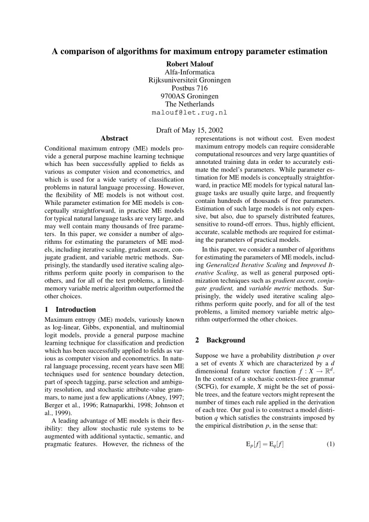
A comparison of algorithms for maximum entropy parameter estimation Robert Malouf Alfa-Informatica Rijksuniversiteit Groningen Postbus 716 9700AS Groningen The Netherlands malouf@let.rug.nl Draft of May 15, 2002 Abstract representations is not without cost. Even modest maximum entropy models can require considerable Conditional maximum entropy (ME) models pro- computational resources and very large quantities of vide a general purpose machine learning technique annotated training data in order to accurately esti- which has been successfully applied to fields as mate the model’s parameters. While parameter es- various as computer vision and econometrics, and timation for ME models is conceptually straightfor- which is used for a wide variety of classification ward, in practice ME models for typical natural lan- problems in natural language processing. However, guage tasks are usually quite large, and frequently the flexibility of ME models is not without cost. contain hundreds of thousands of free parameters. While parameter estimation for ME models is con- Estimation of such large models is not only expen- ceptually straightforward, in practice ME models sive, but also, due to sparsely distributed features, for typical natural language tasks are very large, and sensitive to round-off errors. Thus, highly efficient, may well contain many thousands of free parame- accurate, scalable methods are required for estimat- ters. In this paper, we consider a number of algo- ing the parameters of practical models. rithms for estimating the parameters of ME mod- els, including iterative scaling, gradient ascent, con- In this paper, we consider a number of algorithms for estimating the parameters of ME models, includ- jugate gradient, and variable metric methods. Sur- prisingly, the standardly used iterative scaling algo- ing Generalized Iterative Scaling and Improved It- rithms perform quite poorly in comparison to the erative Scaling , as well as general purposed opti- others, and for all of the test problems, a limited- mization techniques such as gradient ascent, conju- memory variable metric algorithm outperformed the gate gradient, and variable metric methods. Sur- other choices. prisingly, the widely used iterative scaling algo- rithms perform quite poorly, and for all of the test 1 Introduction problems, a limited memory variable metric algo- Maximum entropy (ME) models, variously known rithm outperformed the other choices. as log-linear, Gibbs, exponential, and multinomial logit models, provide a general purpose machine 2 Background learning technique for classification and prediction which has been successfully applied to fields as var- Suppose we have a probability distribution p over ious as computer vision and econometrics. In natu- a set of events X which are characterized by a d ral language processing, recent years have seen ME dimensional feature vector function f : X → R d . techniques used for sentence boundary detection, In the context of a stochastic context-free grammar part of speech tagging, parse selection and ambigu- (SCFG), for example, X might be the set of possi- ity resolution, and stochastic attribute-value gram- ble trees, and the feature vectors might represent the mars, to name just a few applications (Abney, 1997; number of times each rule applied in the derivation Berger et al., 1996; Ratnaparkhi, 1998; Johnson et of each tree. Our goal is to construct a model distri- al., 1999). bution q which satisfies the constraints imposed by A leading advantage of ME models is their flex- the empirical distribution p , in the sense that: ibility: they allow stochastic rule systems to be augmented with additional syntactic, semantic, and E p [ f ] = E q [ f ] pragmatic features. However, the richness of the (1)
E STIMATE ( p ) where E p [ f ] is the expected value of the feature vec- θ 0 ← 0 1 tor under the distribution p : 2 k ← 0 E p [ f ] = ∑ p ( x ) f ( x ) 3 repeat compute q ( k ) from θ ( k ) 4 x ∈ X compute update δ ( k ) 5 In general, this problem is ill posed: a wide range θ ( k + 1 ) ← θ ( k ) + δ ( k ) 6 of models will fit the constraints in (1). As a guide k ← k + 1 7 to selecting one that is most appropriate, we can 8 until converged call on Jaynes’ (1957) Principle of Maximum En- return θ ( k ) 9 tropy : “In the absence of additional information, we should assume that all events have equal probabil- ity.” In other words, we should assign the highest Figure 1: General parameter estimation algorithm prior probability to distributions which maximize the entropy: 3 Maximum likelihood estimation H ( q ) = − ∑ Given the parametric form of an ME model in (4), q ( x ) log q ( x ) (2) fitting an ME model to a collection of training data x ∈ X entails finding values for the parameter vector θ This is effectively a problem in constrained opti- which minimize the relative entropy between the mization: we want to find a distribution q which model q θ and the empirical distribution p , or, equiv- maximizes (2) while satisfying the constraints im- alently, which maximize the log likelihood: posed by (1). It can be straightforwardly shown L ( θ ) = ∑ p ( x , y ) log q ( y | x , θ ) (Jaynes, 1957; Good, 1963; Campbell, 1970) that (5) x , y the solution to this problem has the parametric form: The gradient of the log likelihood function, or the θ T f ( x ) � � exp vector of its first derivatives with respect to the pa- q θ ( x ) = (3) ∑ y ∈ X exp ( θ T f ( y )) rameter θ is: G ( θ ) = ∑ p ( x , y ) f ( y ) − ∑ where θ is a d -dimensional parameter vector and p ( x ) q ( y | x , θ ) f ( y ) θ T f ( x ) is the inner product of the parameter vector x , y x , y and a feature vector. or, simply: One complication which makes models of this form difficult to apply to problems in natural lan- G ( θ ) = E p [ f ] − E q [ f ] (6) guage processing is that the events space X is often very large or even infinite, making the denominator Since the likelihood function (5) is concave over in (3) impossible to compute. One modification we the parameter space, it has a global maximum where can make to avoids this problem is to consider con- the gradient is zero. Unfortunately, simply setting G ( θ ) = 0 and solving for θ does not yield a closed ditional probability distributions instead (Berger et al., 1996; Chi, 1998; Johnson et al., 1999). Suppose form solution, so we proceed iteratively, following now that in addition to the event space X and the the general algorithm in Figure 1. At each step, we adjust an estimate of the parameters θ ( k ) to a new es- feature function f , we have also a set of contexts timate θ ( k + 1 ) based on the divergence between the W and a function Y which partitions the members estimated probability distribution q ( k ) and the em- of X . In our SCFG example, W might be the set of possible strings of words, and Y ( w ) the set of trees pirical distribution p . We continue until successive whose yield is w ∈ W . Computing the conditional improvements fail to yield a sufficiently large de- probability q θ ( x | w ) of an event x in context w as crease in the divergence. While all parameter estimation algorithms we θ T f ( x ) � � exp will consider take the same general form, the q θ ( x | w ) = (4) method for computing the updates δ ( k ) at search step ∑ y ∈ Y ( w ) exp ( θ T f ( y )) differs substantially. As we shall see, this difference now involves evaluating a more much tractable sum can have a dramatic impact on the number of up- in the denominator. dates required to reach convergence.
Recommend
More recommend
Explore More Topics
Stay informed with curated content and fresh updates.
