A comparison between landmarking and joint modeling for producing - PowerPoint PPT Presentation
A comparison between landmarking and joint modeling for producing predictions using longitudinal outcomes Dimitris Rizopoulos, Magdalena Murawska, Eleni-Rosalina Andrinopoulou, Emmanuel Lesaffre and Johanna J.M. Takkenberg Department of
A comparison between landmarking and joint modeling for producing predictions using longitudinal outcomes Dimitris Rizopoulos, Magdalena Murawska, Eleni-Rosalina Andrinopoulou, Emmanuel Lesaffre and Johanna J.M. Takkenberg Department of Biostatistics, Erasmus Medical Center m.murawska@erasmusmc.nl BAYES 2013 , May 21-23, 2013
Dynamic Prediction • Use repeated measurements of specific biomarkers to assess risk of death • Example: CD4 in HIV study • Dynamic prediction: update of survival probability as more measurements are available • We compare two approaches for producing dynamic predictions of survival probabilities • landmarking (van Houwelingen and Putter, 2011) • joint modeling (Rizopoulos, 2012) Erasmus MC, Rotterdam – May 21-23, 2013 1/25
Joint Model Approach • Joint Model Approach: • reconstructs true evolution of biomarker • uses the true values of biomarker in survival model Erasmus MC, Rotterdam – May 21-23, 2013 2/25
Erasmus MC, Rotterdam – May 21-23, 2013 3/25
Joint Model Approach • Two submodels for longitudinal and survival processes • For continuous longitudinal markers usually a linear mixed model is used: y i ( t ) = m i ( t ) + ϵ i ( t ) = x T i ( t ) β + z T i ( t ) b i + ϵ i ( t ) m i ( t ) - true value of the longitudinal marker at time t β - vector of the fixed-effects parameters b i ∼ N (0 , D ) -vector of random effects x i ( t ) and z i ( t ) - design matrices for the fixed and random effects ϵ i ( t ) - measurement error, ϵ i ( t ) ∼ N (0 , σ 2 ) Erasmus MC, Rotterdam – May 21-23, 2013 4/25
Joint Model Approach • For survival process standard relative risk model λ i ( t ) = λ 0 ( t ) exp( α T f ( t, b i ) + γ T v i ) • shares some common (time-dependent) term f ( t, b i ) , with longitudinal model v i - vector of baseline covariates, γ - vector of associated coefficients α - measure the strength of association between longitudinal and survival processes Erasmus MC, Rotterdam – May 21-23, 2013 5/25
Joint Model Approach • Based on fitted model dynamic predictions for new subject k constructed • We predict conditional probability of surviving time u > t given that subject k has survived up to t : S k ( u | t ) = Pr ( T ∗ k > u | T ∗ k > t, Y k ( t )) Y k ( t ) - longitudinal profile for subject k at time t , T ∗ - true survival time • S k ( u | t ) can be written as Bayesian posterior expectation: ∫ Pr ( T ∗ k > u | T ∗ S k ( u | t ) = k > t, Y k ( t ) , S n ; θ ) p ( θ | S n ) dθ (*) θ - vector of parameters from joint model, S n - a sample of size n on which joint model was fitted Erasmus MC, Rotterdam – May 21-23, 2013 6/25
Joint Model Approach • First part of the integrant (*) can be written as: Pr ( T ∗ k > u | T ∗ k > t, Y k ( t ) , S n ; θ ) ∫ Pr ( T k < u | T ∗ k > t, b k ; θ ) × p ( b k | T ∗ = k > t, Y k ( t ) , θ ) db k • Monte Carlo approach used to compute S k ( u | t ) for patient k and S k ( u | t ′ ) updated for every time point t ′ > t Erasmus MC, Rotterdam – May 21-23, 2013 7/25
Landmark Approach • Landmark method simplifies the longitudinal history Y k ( t ) to the last value y k ( t ) • Dynamic predictions obtained by adjusting the risk set and refitting Cox model: • landmark time t L chosen • for t L landmark data set L L constructed: selecting individuals at risk at t L • Cox model fitted for L L • Advantage of JM approach: possibility of defining different association structure between longitudinal and survival processes Erasmus MC, Rotterdam – May 21-23, 2013 8/25
Motivating Data set • PBC study conducted by Mayo Clinic between 1974 and 1984 • For patients with PBC serum bilirubin is known to be a good marker of progression • Aim: find which characteristics of serum bilirubin profile are most predictive for death • Longitudinal serum bilirubin level Y i ( u ) modeled by mixed effects model • natural cubic splines to account for nonlinear character of marker evolution • interaction terms between B-spline basis and treatment group to model different trajectories for 2 treatment groups Erasmus MC, Rotterdam – May 21-23, 2013 9/25
Motivating Data set • For survival process standard relative risk model with different forms of the association structure: I λ i ( t ) = λ 0 ( t ) exp { γ T v i + α 1 m i ( t ) } II λ i ( t ) = λ 0 ( t ) exp { γ T v i + α 1 m i ( t ) + α 2 m ′ i ( t ) } ∫ t { } γ T v i + α 1 III λ i ( t ) = λ 0 ( t ) exp m i ( s ) ds 0 IV λ i ( t ) = λ 0 ( t ) exp { γ T v i + α T b i } . (1) Baseline hazard λ 0 ( t ) modeled parametrically using Weibull distribution, i.e: λ 0 ( t ) = ϕt ϕ − 1 Erasmus MC, Rotterdam – May 21-23, 2013 10/25
PBC Data • Differences between prediction from joint models I-IV and landmark approach observed • Different joint models compared using DIC criterion → best Model I (td-value) Erasmus MC, Rotterdam – May 21-23, 2013 11/25
1.0 40 0.8 30 Serum Bilirubin Level Survival Probability 0.6 20 td−value 0.4 td−both area r−effects 10 LM−value 0.2 0 0.0 0 0.5 5 10 Time Erasmus MC, Rotterdam – May 21-23, 2013 12/25
1.0 40 0.8 30 Serum Bilirubin Level Survival Probability 0.6 20 td−value 0.4 td−both area r−effects 10 LM−value 0.2 0 0.0 0 1 5 10 Time Erasmus MC, Rotterdam – May 21-23, 2013 13/25
1.0 40 0.8 30 Serum Bilirubin Level Survival Probability 0.6 20 td−value 0.4 td−both area r−effects 10 LM−value 0.2 0 0.0 0 2.1 5 10 Time Erasmus MC, Rotterdam – May 21-23, 2013 14/25
1.0 40 0.8 30 Serum Bilirubin Level Survival Probability 0.6 20 td−value 0.4 td−both area r−effects 10 LM−value 0.2 0 0.0 0 4.9 10 Time Erasmus MC, Rotterdam – May 21-23, 2013 15/25
1.0 40 0.8 30 Serum Bilirubin Level Survival Probability 0.6 20 td−value 0.4 td−both area r−effects 10 LM−value 0.2 0 0.0 0 5 5.9 10 Time Erasmus MC, Rotterdam – May 21-23, 2013 16/25
Discrimination • Focus on time interval when the occurence of event is of interest ( t, t + ∆ t ] • Based on the model we would like to dicriminate between patients who are going to exprience the event in that interval from patients who will not • For the first group physiscian can take action to improve survival during ( t, t + ∆ t ] • For c in [0 , 1] we define S k ( u | t ) ≤ c as success and S k ( u | t ) > c as failure • Then sensitivity is defined as: Pr { S k ( u | t ) ≤ c | T ∗ k ∈ ( t, t + ∆ t ] } • And specificity as: Pr { S k ( u | t ) > c | T ∗ k > t + ∆ t } Erasmus MC, Rotterdam – May 21-23, 2013 17/25
Discrimination • For random pair of subjects i, j that have measurments up to t discrimination capability of joint model can be assesed by area under ROC curve (AUC) obtained by varying c : AUC ( t, ∆ t ) = Pr [ S i ( u | t ) < S j ( u | t ) | { T ∗ i ∈ ( t, t + ∆ t ] } ∪ { T ∗ j > t + ∆ t } ] • Model will assign higher probability of surviving longer that t + ∆ t for subject j who did not experience event • To summarize model discrimination power weigthed average of AUCs used: ∫ ∫ ∞ / ∞ C ∆ t dyn = AUC ( t, ∆ t } Pr {E ( t ) } dt Pr {E ( t ) } dt (dynamic concordance index) 0 0 E ( t ) = [ { T ∗ i ∈ ( t, t + ∆ t ] } ∪ { T ∗ j > t + ∆ t } ] Pr {E ( t ) } -probability that pair { i, j } comparable at t Erasmus MC, Rotterdam – May 21-23, 2013 18/25
Discrimination • C ∆ t dyn depends on ∆ t • In practice: ∑ 15 AUC ( t q , ∆ t ) × ˆ ˆ ω q Pr {E ( t q ) } ∆ t q =1 ˆ C dyn = ∑ 15 ω q ˆ Pr {E ( t q ) } q =1 ω q -weights for 15 Gauss-Kronrod quadrature points on (0 , t max ) Pr {E ( t ) } = { ˆ ˆ S ( t q ) − ˆ S ( t q + ∆ t ) } ˆ S ( t q + ∆ t ) ˆ S ( · ) -Kaplan-Meier estimator of marginal survival function S ( · ) Erasmus MC, Rotterdam – May 21-23, 2013 19/25
Discrimination • AUC is estimated as: ∑ ∑ n n I { ˆ S i ( t + ∆ t | t ) < ˆ S j ( t + ∆ t | t ) } × I { Ω ij ( t ) } i = i j =1 ,j ̸ = i ˆ AUC ( t q , ∆ t ) = ∑ ∑ n n I { Ω ij ( t ) } i = i j =1 ,j ̸ = i • Comparable pairs are those that satisfy: Ω ij ( t ) = [ { T i ∈ ( t, t + ∆ t ] } ∩ { δ i = 1 } ] ∩ { T j > t + ∆ t } or Ω ij ( t ) = [ { T i ∈ ( t, t + ∆ t ] } ∩ { δ i = 1 } ] ∩ [ { T j = t + ∆ t } ∩ { δ j = 0 } ] Erasmus MC, Rotterdam – May 21-23, 2013 20/25
Calibration • Expected Prediction Error (Henderson et al 2002): PE ( u | t ) = E [ L { N i ( u ) − S i ( u | t ) } ] N i ( u ) = I ( T ∗ i > u ) L ( · ) -loss function (absolute or square loss) PE ( u | t ) = {R ( t ) } − 1 ∑ ˆ I ( T i > u ) L { 1 − ˆ S ( u | t ) } + δ i I ( T i < u ) L { 0 − ˆ S ( u | t ) } i : T i ≥ t +(1 − δ i ) I ( T i < u )[ ˆ S i ( u | T i ) L { 1 − ˆ S ( u | t ) } + { 1 − ˆ S ( u | T i ) } L { 0 − ˆ S ( u | t ) } ] R ( t ) -number of subjects at risk at t Erasmus MC, Rotterdam – May 21-23, 2013 21/25
Recommend
More recommend
Explore More Topics
Stay informed with curated content and fresh updates.
