a , b y i a x i b 2 . min (2) 2. Some Useful Asymptotic - PowerPoint PPT Presentation
A Course in Applied Econometrics 1 . Reminders About Means , Medians , and Quantiles Lecture 17 : Quantile Methods Linear Population Model, where is K 1: y x u . (1) Jeff Wooldridge IRP Lectures, UW Madison, August
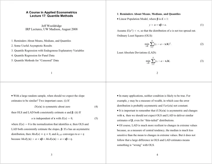
A Course in Applied Econometrics 1 . Reminders About Means , Medians , and Quantiles Lecture 17 : Quantile Methods � Linear Population Model, where � is K � 1: y � � � x � � u . (1) Jeff Wooldridge IRP Lectures, UW Madison, August 2008 Assume E � u 2 � � � , so that the distribution of u is not too spread out. Ordinary Least Squares (OLS): 1. Reminders About Means, Medians, and Quantiles N a , b � � y i � a � x i b � 2 . min (2) 2. Some Useful Asymptotic Results i � 1 3. Quantile Regression with Endogenous Explanatory Variables Least Absolute Deviations (LAD): 4. Quantile Regression for Panel Data N a , b � 5. Quantile Methods for “Censored” Data | y i � a � x i b |. min (3) i � 1 1 2 � With a large random sample, when should we expect the slope � In many applications, neither condition is likely to be true. For estimates to be similar? Two important cases. (i) If example, y may be a measure of wealth, in which case the error distribution is probably asymmetric and Var � u | x � not constant. D � u | x � is symmetric about zero (4) � It is important to remember that if D � u | x � is asymmetric and changes then OLS and LAD both consistently estimate � and � . (ii) If with x , then we should not expect OLS and LAD to deliver similar u is independent of x with E � u � � 0, (5) estimates of � , even for “thin-tailed” distributions. where E � u � � 0 is the normalization that identifies � , then OLS and � Of course, LAD is much more resilient to changes in extreme values LAD both consistently estimate the slopes, � . If u has an asymmetric because, as a measure of central tendency, the median is much less � LAD converges to � � � distribution, then Med � u � � � � 0, and � sensitive than the mean to changes in extreme values. But it does not because Med � y | x � � � � x � � Med � u | x � � � � x � � � . follow that a large difference in OLS and LAD estimates means something is “wrong” with OLS. 3 4
� Advantage for median over mean: median passes through monotonic � What can we add so that LAD estimates something of interest in (7)? functions. If log � y � � � � x � � u and Med � u | x � � 0, then If u i is a vector, then its distribution conditional on x i is centrally Med � y | x � � exp � Med � log � y � | x �� � exp � � � x � � . By contrast, we symmetric if D � u i | x i � � D � � u i | x i � ,which implies that, if g i is any � u i | x i � has a univariate distribution that is cannot generally find E � y | x � � exp � � � x � � E � exp � u � | x � . vector function of x i , D � g i � But expectation has useful properties that the median does not: symmetric about zero. This implies E � u i | x i � � 0 . � Write linearity and the law of iterated expectations. If y i � a i � x i b i y i � � � x i � � � a i � � � � x i � b i � � � . (6) (8) and � a i , b i � is independent of x i , then If c i � � a i , b i � given x i is centrally symmetric then LAD applied to the usual model y i � � � x i � � u i consistently estimates � and � . E � y i | x i � � E � a i | x i � � x i E � b i | x i � � � � x i � , (7) where � � E � a i � and � � E � b i � . OLS is consistent for � and � . 5 6 � For 0 � � � 1, q � � � is the � th quantile of y i if P � y i � q � � �� � � and 2 . Some Useful Asymptotic Results P � y i � q � � �� � 1 � � . What Happens if the Quantile Function is Misspecified ? � Let covariates affect quantiles. Under linearity, � Property of OLS: if � � and � � are the plims from the OLS regression y i on 1, x i then these provide the smallest mean squared error Quant � � y i | x i � � � � � � � x i � � � � . (9) approximation to E � y | x � � � � x � in that � � � , � � � solve Under (9), consistent estimators of � � � � and � � � � are obtained by � , � E �� � � x � � � � x � � 2 � . min (11) minimizing the “check” function: N � can be equal to or Under restrictive assumptions on distribution of x , � j � � � , � � � K � c � � y i � � � x i � � , min (10) i � 1 proportionl to average partial effects. where c � � u � � � � 1 � u � 0 � � � 1 � � � 1 � u � 0 �� | u | � � � � 1 � u � 0 �� u and 1 ��� is the “indicator function.” 7 8
� Linear quantile formulation has been viewed by several authors as an Computing Standard Errors � For given � , write approximation. Recently, Angrist, Chernozhukov, and Fernandez-Val (2006) characterized the probability limit of the quantile regression y i � x i � � u i , Quant � � u i | x i � � 0, (14) estimator. Absorb the intercept into x and let � � � � be the solution to the � be the quantile estimator. Define quantile residuals and let � population quantile regression problem. ACF show that � � � � solves � . Generally, � � � � is asymptotically normal with û i � y i � x i � N � � E � w � � x , � �� q � � x � � x � �� 2 � , min (12) asymptotic variance A � 1 BA � 1 ,where � A � E � f u � 0| x i � x i � x i � where the weight function w � � x , � � is (15) w � � x , � � � � 1 and � 1 � u � f y | x � u x � � � 1 � u � q � � x � | x � du . (13) 0 � x i � . B � � � 1 � � � E � x i (16) 9 10 � If the quantile function is actually linear, a consistent estimator of B � If u i and x i are independent, � � � � � � � 1 � � � is Avar N � � � f u � 0 �� 2 � E � x i � x i �� � 1 , (19) N � 1 � N � � � � 1 � � � � x i B x i . (17) � � is estimated as and Avar � � i � 1 � 1 N � 1 � N Generally, a consistent estimator of A is (Powell (1991)) � � � � � 1 � � � � x i Avar � � x i , (20) � u � 0 �� 2 � f i � 1  � � 2 Nh N � � 1 � N � x i , 1 � | û i | � h N � x i (18) � u � 0 � is the histogram estimator where, say, f i � 1 � u � 0 � � � 2 Nh N � � 1 � N where � h N � 0 � is a nonrandom sequence shrinking to zero as N � � 1 � | û i | � h N � . f (21) N h N � � . For example, h N � aN � 1/3 for any a � 0. Might use a with i � 1 smoothed version so that all residuals contribute. Estimate in (20) is commonly reported (by, say, Stata). 11 12
� If the quantile function is misspecified, the “robust” form based on � Hahn (1995, 1997) shows that the nonparametric bootstrap and the (20), is not valid. In the generalized linear models literature, distinction Bayesian bootstrap generally provide consistent estimates of the fully between “fully robust” variance estimator (mean correctly specified) robust variance without claims about the conditional quantile being and a “semi-robust” estimator (mean might be misspecified). correct. Bootstrap does not provide “asymptotic refinements” for � For quantile regression, a fully robust variance requires a different testing and confidence intervals. � ACF provide the covariance function for the process estimator of B . Kim and White (2002) and Angrist, Chernozhukov, and � � � � : � � � � 1 � � � for some � � 0, which can be used to test � � Fernández-Val (2006) show hypotheses jointly across multiple quantiles (including all quantiles at N N � 1 � � � � x i B � � � 1 � û i � 0 �� 2 x i (22) once). i � 1 � Example using Abadie (2003). These are nonrobust standard errors. � 1 with  given by (18). � 1 B � � �  �  is consistent, and then Avar � � nettfa is net total financial assets. 13 14 3 . Quantile Regression with Endogenous Explanatory Variables Dependent Variable: nettfa � Suppose Explanatory Variable Mean (OLS) .25 Quantile Median (LAD) .75 Quantile inc .783 .0713 .324 .798 y 1 � z 1 � 1 � � 1 y 2 � u 1 , (23) � .104 � � .0072 � � .012 � � .025 � where z is exogenous and y 2 is endogenous – whatever that means in � 1.568 � .244 � 1.386 age .0336 the context of quantile regression. � 1.076 � � .0955 � � .146 � � .287 � � Amemiya’s (1982) two-stage LAD estimator: reduced form for y 2 , age 2 .0284 .0004 .0048 .0242 � .0138 � � .0011 � � .0017 � � .0034 � y 2 � z � 2 � v 2 . (24) e 401 k 6.837 1.281 2.598 4.460 First step applies OLS or LAD to (24), and gets fitted values, � 2.173 � � .263 � � .404 � � .801 � � 2 . These are inserted for y i 2 to give LAD of y i 1 on z i 1 , � i 2 . y i 2 � z i � N 2,017 2,017 2,017 2,017 2SLAD relies on symmetry of the composite error � 1 v 2 � u 1 given z . 15 16
Recommend
More recommend
Explore More Topics
Stay informed with curated content and fresh updates.
