9. Numerical linear algebra background matrix structure and - PowerPoint PPT Presentation
Convex Optimization Boyd & Vandenberghe 9. Numerical linear algebra background matrix structure and algorithm complexity solving linear equations with factored matrices LU, Cholesky, LDL T factorization block elimination and
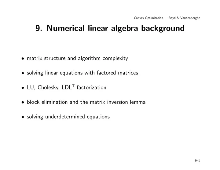
Convex Optimization — Boyd & Vandenberghe 9. Numerical linear algebra background • matrix structure and algorithm complexity • solving linear equations with factored matrices • LU, Cholesky, LDL T factorization • block elimination and the matrix inversion lemma • solving underdetermined equations 9–1
Matrix structure and algorithm complexity cost (execution time) of solving Ax = b with A ∈ R n × n • for general methods, grows as n 3 • less if A is structured (banded, sparse, Toeplitz, . . . ) flop counts • flop (floating-point operation): one addition, subtraction, multiplication, or division of two floating-point numbers • to estimate complexity of an algorithm: express number of flops as a (polynomial) function of the problem dimensions, and simplify by keeping only the leading terms • not an accurate predictor of computation time on modern computers • useful as a rough estimate of complexity Numerical linear algebra background 9–2
vector-vector operations ( x , y ∈ R n ) • inner product x T y : 2 n − 1 flops (or 2 n if n is large) • sum x + y , scalar multiplication αx : n flops matrix-vector product y = Ax with A ∈ R m × n • m (2 n − 1) flops (or 2 mn if n large) • 2 N if A is sparse with N nonzero elements • 2 p ( n + m ) if A is given as A = UV T , U ∈ R m × p , V ∈ R n × p matrix-matrix product C = AB with A ∈ R m × n , B ∈ R n × p • mp (2 n − 1) flops (or 2 mnp if n large) • less if A and/or B are sparse • (1 / 2) m ( m + 1)(2 n − 1) ≈ m 2 n if m = p and C symmetric Numerical linear algebra background 9–3
Linear equations that are easy to solve diagonal matrices ( a ij = 0 if i � = j ): n flops x = A − 1 b = ( b 1 /a 11 , . . . , b n /a nn ) lower triangular ( a ij = 0 if j > i ): n 2 flops x 1 := b 1 /a 11 x 2 := ( b 2 − a 21 x 1 ) /a 22 x 3 := ( b 3 − a 31 x 1 − a 32 x 2 ) /a 33 . . . x n := ( b n − a n 1 x 1 − a n 2 x 2 − · · · − a n,n − 1 x n − 1 ) /a nn called forward substitution upper triangular ( a ij = 0 if j < i ): n 2 flops via backward substitution Numerical linear algebra background 9–4
orthogonal matrices: A − 1 = A T • 2 n 2 flops to compute x = A T b for general A • less with structure, e.g. , if A = I − 2 uu T with � u � 2 = 1 , we can compute x = A T b = b − 2( u T b ) u in 4 n flops permutation matrices: � 1 j = π i a ij = 0 otherwise where π = ( π 1 , π 2 , . . . , π n ) is a permutation of (1 , 2 , . . . , n ) • interpretation: Ax = ( x π 1 , . . . , x π n ) • satisfies A − 1 = A T , hence cost of solving Ax = b is 0 flops example: 0 1 0 0 0 1 A − 1 = A T = , A = 0 0 1 1 0 0 1 0 0 0 1 0 Numerical linear algebra background 9–5
The factor-solve method for solving Ax = b • factor A as a product of simple matrices (usually 2 or 3): A = A 1 A 2 · · · A k ( A i diagonal, upper or lower triangular, etc) • compute x = A − 1 b = A − 1 k · · · A − 1 2 A − 1 1 b by solving k ‘easy’ equations A 1 x 1 = b, A 2 x 2 = x 1 , . . . , A k x = x k − 1 cost of factorization step usually dominates cost of solve step equations with multiple righthand sides Ax 1 = b 1 , Ax 2 = b 2 , . . . , Ax m = b m cost: one factorization plus m solves Numerical linear algebra background 9–6
LU factorization every nonsingular matrix A can be factored as A = PLU with P a permutation matrix, L lower triangular, U upper triangular cost: (2 / 3) n 3 flops Solving linear equations by LU factorization. given a set of linear equations Ax = b , with A nonsingular. 1. LU factorization. Factor A as A = P LU ( (2 / 3) n 3 flops). 2. Permutation. Solve P z 1 = b ( 0 flops). 3. Forward substitution. Solve Lz 2 = z 1 ( n 2 flops). 4. Backward substitution. Solve Ux = z 2 ( n 2 flops). cost: (2 / 3) n 3 + 2 n 2 ≈ (2 / 3) n 3 for large n Numerical linear algebra background 9–7
sparse LU factorization A = P 1 LUP 2 • adding permutation matrix P 2 offers possibility of sparser L , U (hence, cheaper factor and solve steps) • P 1 and P 2 chosen (heuristically) to yield sparse L , U • choice of P 1 and P 2 depends on sparsity pattern and values of A • cost is usually much less than (2 / 3) n 3 ; exact value depends in a complicated way on n , number of zeros in A , sparsity pattern Numerical linear algebra background 9–8
Cholesky factorization every positive definite A can be factored as A = LL T with L lower triangular cost: (1 / 3) n 3 flops Solving linear equations by Cholesky factorization. given a set of linear equations Ax = b , with A ∈ S n ++ . 1. Cholesky factorization. Factor A as A = LL T ( (1 / 3) n 3 flops). 2. Forward substitution. Solve Lz 1 = b ( n 2 flops). 3. Backward substitution. Solve L T x = z 1 ( n 2 flops). cost: (1 / 3) n 3 + 2 n 2 ≈ (1 / 3) n 3 for large n Numerical linear algebra background 9–9
sparse Cholesky factorization A = PLL T P T • adding permutation matrix P offers possibility of sparser L • P chosen (heuristically) to yield sparse L • choice of P only depends on sparsity pattern of A (unlike sparse LU) • cost is usually much less than (1 / 3) n 3 ; exact value depends in a complicated way on n , number of zeros in A , sparsity pattern Numerical linear algebra background 9–10
LDL T factorization every nonsingular symmetric matrix A can be factored as A = PLDL T P T with P a permutation matrix, L lower triangular, D block diagonal with 1 × 1 or 2 × 2 diagonal blocks cost: (1 / 3) n 3 • cost of solving symmetric sets of linear equations by LDL T factorization: (1 / 3) n 3 + 2 n 2 ≈ (1 / 3) n 3 for large n • for sparse A , can choose P to yield sparse L ; cost ≪ (1 / 3) n 3 Numerical linear algebra background 9–11
Equations with structured sub-blocks � � � � � � A 11 A 12 x 1 b 1 = (1) A 21 A 22 x 2 b 2 • variables x 1 ∈ R n 1 , x 2 ∈ R n 2 ; blocks A ij ∈ R n i × n j • if A 11 is nonsingular, can eliminate x 1 : x 1 = A − 1 11 ( b 1 − A 12 x 2 ) ; to compute x 2 , solve ( A 22 − A 21 A − 1 11 A 12 ) x 2 = b 2 − A 21 A − 1 11 b 1 Solving linear equations by block elimination. given a nonsingular set of linear equations (1), with A 11 nonsingular. 1. Form A − 1 11 A 12 and A − 1 11 b 1 . 11 A 12 and ˜ 2. Form S = A 22 − A 21 A − 1 b = b 2 − A 21 A − 1 11 b 1 . 3. Determine x 2 by solving Sx 2 = ˜ b . 4. Determine x 1 by solving A 11 x 1 = b 1 − A 12 x 2 . Numerical linear algebra background 9–12
dominant terms in flop count • step 1: f + n 2 s ( f is cost of factoring A 11 ; s is cost of solve step) 2 n 1 (cost dominated by product of A 21 and A − 1 • step 2: 2 n 2 11 A 12 ) • step 3: (2 / 3) n 3 2 total: f + n 2 s + 2 n 2 2 n 1 + (2 / 3) n 3 2 examples • general A 11 ( f = (2 / 3) n 3 1 , s = 2 n 2 1 ): no gain over standard method #flops = (2 / 3) n 3 1 + 2 n 2 1 n 2 + 2 n 2 2 n 1 + (2 / 3) n 3 2 = (2 / 3)( n 1 + n 2 ) 3 • block elimination is useful for structured A 11 ( f ≪ n 3 1 ) for example, diagonal ( f = 0 , s = n 1 ): #flops ≈ 2 n 2 2 n 1 + (2 / 3) n 3 2 Numerical linear algebra background 9–13
Structured matrix plus low rank term ( A + BC ) x = b • A ∈ R n × n , B ∈ R n × p , C ∈ R p × n • assume A has structure ( Ax = b easy to solve) first write as � � � � � � A B x b = C − I y 0 now apply block elimination: solve ( I + CA − 1 B ) y = CA − 1 b, then solve Ax = b − By this proves the matrix inversion lemma: if A and A + BC nonsingular, ( A + BC ) − 1 = A − 1 − A − 1 B ( I + CA − 1 B ) − 1 CA − 1 Numerical linear algebra background 9–14
example: A diagonal, B, C dense • method 1: form D = A + BC , then solve Dx = b cost: (2 / 3) n 3 + 2 pn 2 • method 2 (via matrix inversion lemma): solve ( I + CA − 1 B ) y = CA − 1 b, (2) then compute x = A − 1 b − A − 1 By total cost is dominated by (2): 2 p 2 n + (2 / 3) p 3 ( i.e. , linear in n ) Numerical linear algebra background 9–15
Underdetermined linear equations if A ∈ R p × n with p < n , rank A = p , x | z ∈ R n − p } { x | Ax = b } = { Fz + ˆ • ˆ x is (any) particular solution • columns of F ∈ R n × ( n − p ) span nullspace of A • there exist several numerical methods for computing F (QR factorization, rectangular LU factorization, . . . ) Numerical linear algebra background 9–16
Recommend


More recommend
Explore More Topics
Stay informed with curated content and fresh updates.