8 Approximate inference in switching linear dynamical systems using - PDF document

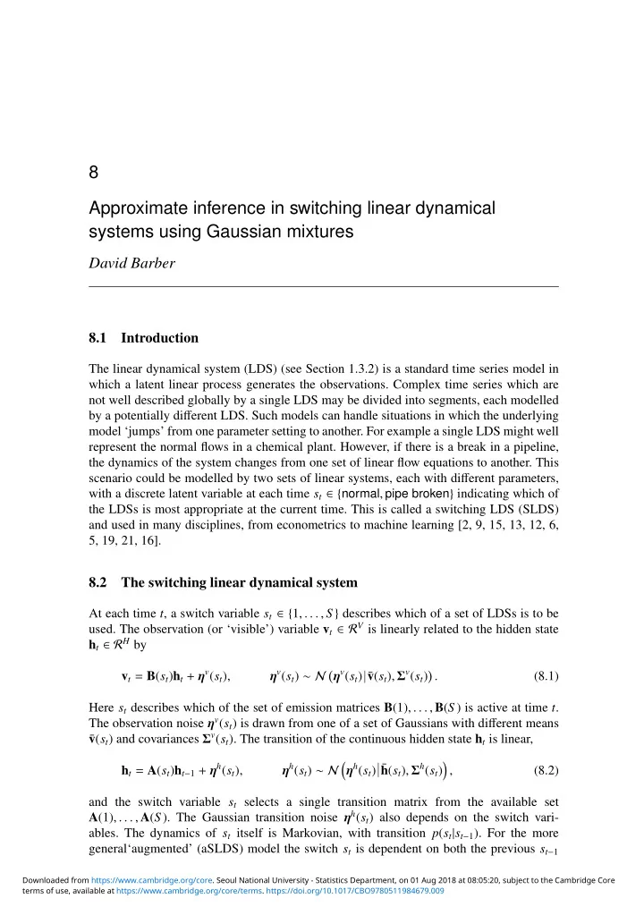
8 Approximate inference in switching linear dynamical systems using Gaussian mixtures David Barber 8.1 Introduction The linear dynamical system (LDS) (see Section 1.3.2) is a standard time series model in which a latent linear process generates the observations. Complex time series which are not well described globally by a single LDS may be divided into segments, each modelled by a potentially di ff erent LDS. Such models can handle situations in which the underlying model ‘jumps’ from one parameter setting to another. For example a single LDS might well represent the normal flows in a chemical plant. However, if there is a break in a pipeline, the dynamics of the system changes from one set of linear flow equations to another. This scenario could be modelled by two sets of linear systems, each with di ff erent parameters, with a discrete latent variable at each time s t ∈ { normal , pipe broken } indicating which of the LDSs is most appropriate at the current time. This is called a switching LDS (SLDS) and used in many disciplines, from econometrics to machine learning [2, 9, 15, 13, 12, 6, 5, 19, 21, 16]. 8.2 The switching linear dynamical system At each time t , a switch variable s t ∈ { 1 , . . . , S } describes which of a set of LDSs is to be used. The observation (or ‘visible’) variable v t ∈ R V is linearly related to the hidden state h t ∈ R H by v ( s t ) , Σ v ( s t ) � . v t = B ( s t ) h t + η v ( s t ) , η v ( s t ) ∼ N � η v ( s t ) ¯ (8.1) Here s t describes which of the set of emission matrices B (1) , . . . , B ( S ) is active at time t . The observation noise η v ( s t ) is drawn from one of a set of Gaussians with di ff erent means v ( s t ) and covariances Σ v ( s t ). The transition of the continuous hidden state h t is linear, ¯ � η h ( s t ) ¯ � h t = A ( s t ) h t − 1 + η h ( s t ) , η h ( s t ) ∼ N h ( s t ) , Σ h ( s t ) , (8.2) and the switch variable s t selects a single transition matrix from the available set A (1) , . . . , A ( S ). The Gaussian transition noise η h ( s t ) also depends on the switch vari- ables. The dynamics of s t itself is Markovian, with transition p ( s t | s t − 1 ). For the more general‘augmented’ (aSLDS) model the switch s t is dependent on both the previous s t − 1 Downloaded from https://www.cambridge.org/core. Seoul National University - Statistics Department, on 01 Aug 2018 at 08:05:20, subject to the Cambridge Core terms of use, available at https://www.cambridge.org/core/terms. https://doi.org/10.1017/CBO9780511984679.009

Inference in switching linear systems using mixtures 167 s 1 s 2 s 3 s 4 Figure 8.1 The independence structure of the aSLDS. Square nodes s t denote discrete switch variables; h t are continu- ous latent / hidden variables, and v t continuous observed / vis- h 1 h 2 h 3 h 4 ible variables. The discrete state s t determines which linear dynamical system from a finite set of linear dynamical sys- tems is operational at time t . In the SLDS links from h to s are not normally considered. v 1 v 2 v 3 v 4 and h t − 1 . The probabilistic model defines a joint distribution, see Fig. 8.1, T � p ( v 1: T , h 1: T , s 1: T ) = p ( v t | h t , s t ) p ( h t | h t − 1 , s t ) p ( s t | h t − 1 , s t − 1 ) , t = 1 v ( s t ) + B ( s t ) h t , Σ v ( s t )) , p ( v t | h t , s t ) = N ( v t ¯ � � h t ¯ h ( s t ) + A ( s t ) h t − 1 , Σ h ( s t ) p ( h t | h t − 1 , s t ) = N . At time t = 1, p ( s 1 | h 0 , s 0 ) denotes the prior p ( s 1 ), and p ( h 1 | h 0 , s 1 ) denotes p ( h 1 | s 1 ). The SLDS can be thought of as a marriage between a hidden Markov model and an LDS. The SLDS is also called a jump Markov model / process, switching Kalman filter, switching linear Gaussian state space model, conditional linear Gaussian model. 8.2.1 Exact inference is computationally intractable Performing exact filtered and smoothed inference in the SLDS is intractable, scaling expo- nentially with time, see for example [16]. As an informal explanation, consider filtered posterior inference, for which, by analogy with Section 1.4.1 the forward pass is � � p ( s t + 1 , h t + 1 | v 1: t + 1 ) = p ( s t + 1 , h t + 1 | s t , h t , v t + 1 ) p ( s t , h t | v 1: t ) . (8.3) h t s t At time step 1, p ( s 1 , h 1 | v 1 ) = p ( h 1 | s 1 , v 1 ) p ( s 1 | v 1 ) is an indexed Gaussian. At time step 2, due to the summation over the states s 1 , p ( s 2 , h 2 | v 1:2 ) is an indexed set of S Gaussians. In general, at time t , p ( s t , h t | v 1: t ) is an indexed set of S t − 1 Gaussians. Even for small t , the num- ber of components required to exactly represent the filtered distribution is computationally intractable. Analogously, smoothing is also intractable. The origin of the intractability of the SLDS therefore di ff ers from ‘structural intractabil- ity’ since, in terms of the cluster variables x 1: T with x t ≡ ( s t , h t ) and visible variables v 1: T , the graph of the distribution is singly connected. From a purely graph-theoretic view- point, one would therefore envisage no di ffi culty in carrying out inference. Indeed, as we saw above, the derivation of the filtering algorithm is straightforward since the graph of p ( x 1: T , v 1: T ) is singly connected. However, the numerical representation of the messages requires an exponentially increasing number of terms. In order to deal with this intractability, several approximation schemes have been intro- duced, [8, 9, 15, 13, 12]. Here we focus on techniques which approximate the switch conditional posteriors using a limited mixture of Gaussians. Since the exact posterior distributions are mixtures of Gaussians, but with an exponentially large number of com- ponents, the aim is to drop low-weight components such that the resulting limited number of Gaussians still accurately represents the posterior. Downloaded from https://www.cambridge.org/core. Seoul National University - Statistics Department, on 01 Aug 2018 at 08:05:20, subject to the Cambridge Core terms of use, available at https://www.cambridge.org/core/terms. https://doi.org/10.1017/CBO9780511984679.009

168 David Barber 8.3 Gaussian sum filtering Equation (8.3) describes the exact filtering recursion. Whilst the number of mixture com- ponents increases exponentially with time, intuitively one would expect that there is an e ff ective time scale over which the previous visible information is relevant. In general, the influence of ancient observations will be much less relevant than that of recent observa- tions. This suggests that a limited number of components in the Gaussian mixture should su ffi ce to accurately represent the filtered posterior [1]. Our aim is to form a recursion for p ( s t , h t | v 1: t ) using a Gaussian mixture approxi- mation of p ( h t | s t , v 1: t ). Given an approximation of the filtered distribution p ( s t , h t | v 1: t ) ≈ q ( s t , h t | v 1: t ), the exact recursion (8.3) is approximated by � � q ( s t + 1 , h t + 1 | v 1: t + 1 ) = p ( s t + 1 , h t + 1 | s t , h t , v t + 1 ) q ( s t , h t | v 1: t ) . (8.4) h t s t This approximation to the filtered posterior at the next time step will contain S times more components than at the previous time step. Therefore to prevent an exponential explosion in mixture components we need to collapse this mixture in a suitable way. We will deal with this once the new mixture representation for the filtered posterior has been computed. To derive the updates it is useful to break the filtered approximation from Eq. (8.4) into continuous and discrete parts q ( h t , s t | v 1: t ) = q ( h t | s t , v 1: t ) q ( s t | v 1: t ) , (8.5) and derive separate filtered update formulae, as described below. An important remark is that many techniques approximate p ( h t | s t , v 1: t ) using a single Gaussian. Naturally, this gives rise to a mixture of Gaussians for p ( h t | v 1: t ). However, in making a single Gaussian approximation to p ( h t | s t , v 1: t ) the representation of the posterior may be poor. Our aim here is to maintain an accurate approximation to p ( h t | s t , v 1: t ) by using a mixture of Gaussians. 8.3.1 Continuous filtering The exact representation of p ( h t | s t , v 1: t ) is a mixture with S t − 1 components. To retain computational feasibility we approximate this with a limited I -component mixture I � q ( h t | s t , v 1: t ) = q ( h t | i t , s t , v 1: t ) q ( i t | s t , v 1: t ) , i t = 1 where q ( h t | i t , s t , v 1: t ) is a Gaussian parameterised with mean f ( i t , s t ) and covariance F ( i t , s t ). Strictly speaking, we should use the notation f t ( i t , s t ) since, for each time t , we have a set of means indexed by i t , s t , but we drop these dependencies in the notation used here. To find a recursion for the approximating distribution, we first assume that we know the filtered approximation q ( h t , s t | v 1: t ) and then propagate this forwards using the exact dynamics. To do so consider first the exact relation � q ( h t + 1 | s t + 1 , v 1: t + 1 ) = q ( h t + 1 , s t , i t | s t + 1 , v 1: t + 1 ) s t , i t � = q ( h t + 1 | s t , i t , s t + 1 , v 1: t + 1 ) q ( s t , i t | s t + 1 , v 1: t + 1 ) . (8.6) s t , i t Downloaded from https://www.cambridge.org/core. Seoul National University - Statistics Department, on 01 Aug 2018 at 08:05:20, subject to the Cambridge Core terms of use, available at https://www.cambridge.org/core/terms. https://doi.org/10.1017/CBO9780511984679.009