5.3.9 Line detection by local pre-processing operators Special - PowerPoint PPT Presentation

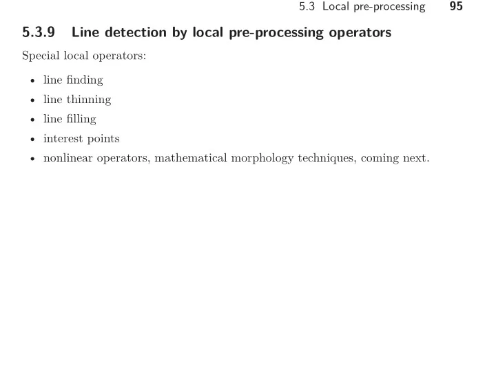
95 5.3 Local pre-processing 5.3.9 Line detection by local pre-processing operators Special local operators: • line finding • line thinning • line filling • interest points • nonlinear operators, mathematical morphology techniques, coming next.

96 5.3 Local pre-processing • edge detector is a general tool not depending on image content • detected edges are to some degree robust – do not depend much on small changes in illumination, viewpoint change, etc. • richer features can be reliably detected • special detectors can outperform simple edge detectors in some classes of appli- cations – Line detectors used to detect linear objects such as dimension lines in engineering drawings or railways or roads in satellite images – corner detectors, interest point detectors used mainly to register two or more images one to the other

97 5.3 Local pre-processing Line finding operators • find very thin curves in the image • assume that curves do not bend sharply • line may be detected by local convolution • four such 3 × 3 kernels detect lines rotated modulo 45 o .       − 1 − 1 − 1 2 − 1 − 1 − 1 2 − 1  ,  ,  , h 1 = 2 2 2 h 2 = − 1 2 − 1 h 3 = − 1 2 − 1 . . .    − 1 − 1 − 1 − 1 − 1 2 − 1 2 − 1 (5.70) • 5 × 5 masks also common • line detectors may produce more lines than needed • non-linear constraints may reduce this

98 5.3 Local pre-processing 5.3.10 Detection of corners (interest points) • finding pairs of corresponding points in two similar images • all possible pairs of pixels should be examined to solve this correspondence problem , — very computationally expensive • process is simplified if correspondence of interest points is used • interest point should have some typical local property • corners are very good interest points • Corner detectors – input – gray-level image – output – values proportional to likelihood that pixel is a corner • Interest points — by thresholding • corners serve better than lines in correspondence problems • due to the aperture problem ? Figure 5.34 : Ambiguity of lines for matching and unambiguity of cor- ners.

99 5.3 Local pre-processing • Edge detectors not stable at corners • gradient at the tip of the corner is ambiguous • this observation is used in corner detectors ? Figure 5.35 : Ambiguity of edge detector at the corner tip. • corner can be defined as a pixel, a small neighborhood of which has two dom- inant and different edge directions • this definition is not precise – isolated point of local intensity maximum or minimum, line endings, or an abrupt change in the curvature of a curve gives a response similar to a corner • yet – such detectors are named corner detectors and are widely used • if “true” corners have to be detected then some additional constraints must be used

100 5.3 Local pre-processing • corner detectors are usually not robust • may be overcome by manual expert supervision or large redundancies to prevent individual errors from dominating the task = many more corners are detected in two or more images than are needed for estimating a transformation sought between these images • Moravec detector [Moravec 77] – simplest • maximal in pixels with high contrast • = corners and sharp edges i +1 j +1 MO( i, j ) = 1 � � � . � � � f ( k, l ) − f ( i, j ) (5.71) 8 k = i − 1 l = j − 1

101 5.3 Local pre-processing • computationally more expensive corner operators give better results – possibly based on facet models • image f approximated in neighborhood of pixel ( i, j ) by cubic polynomial with coefficients c k : f ( i, j ) = c 1 + c 2 x + c 3 y + c 4 x 2 + c 5 x y + c 6 y 2 + c 7 x 3 + c 8 x 2 y + c 9 x y 2 + c 10 y 3 (5.72) • Zuniga–Haralick operator ZH ZH( i, j ) = − 2 ( c 2 2 c 6 − c 2 c 3 c 5 + c 2 3 c 4 ) . (5.73) � 3 / 2 c 2 2 + c 2 � 3 • Kitchen-Rosenfeld KR operator is similar KR( i, j ) = − 2 ( c 2 2 c 6 − c 2 c 3 c 5 + c 2 3 c 4 ) c 2 2 + c 2 3 • ZH operator did outperform the KR corner detector in test images [Haralick and Shapir

102 5.3 Local pre-processing • Harris corner detector [Harris and Stephen 88] improved upon Moravec’s • added differential of the corner score (sum of square differences) • image patch W ∈ f shifted by ∆ x, ∆ y • sum of square differences S between values of the image f given by the patch W and its shifted variant by ∆ x , ∆ y given by: � 2 . � � � S W (∆ x, ∆ y ) = f ( x i , y i ) − f ( x i − ∆ x, y i − ∆ y ) (5.74) x i ∈ W y i ∈ W

103 5.3 Local pre-processing • corner point not suffering from aperture problem • ⇒ high response of S W (∆ x, ∆ y ) for all ∆ x , ∆ y • if the shifted image patch is approximated by the first-order Taylor expansion � ∂f ( x i , y i ) � � ∆ x � , ∂f ( x i , y i ) f ( x i − ∆ x, y i − ∆ y ) ≈ f ( x i , y i ) + (5.75) , ∆ y ∂x ∂y • then minimum of S W (∆ x, ∆ y ) can be obtained analytically

104 5.3 Local pre-processing • substitute this approximation given by equation (5.75) into equation (5.74) 2 � � ∂f ( x i , y i ) � � ∆ x �� , ∂f ( x i , y i ) � � S ( x, y ) = f ( x i , y i ) − f ( x i , y i ) − ∆ y ∂x ∂y x i ∈ W y i ∈ W 2 � � ∂f ( x i , y i ) , ∂f ( x i , y i ) � � ∆ x �� � � = − ∆ y ∂x ∂y x i ∈ W y i ∈ W 2 � � ∂f ( x i , y i ) , ∂f ( x i , y i ) � � �� ∆ x � � = ∆ y ∂x ∂y x i ∈ W y i ∈ W having in mind that u 2 = u ⊤ u �� ∂f � � �� � ∆ x � ∂x � � ∂f ∂f = [∆ x, ∆ y ] ∂x ∂y ∆ y ∂f x i ∈ W y i ∈ W ∂y � ∂f   � � � � ∆ x � ∂x  � � ∂f ∂f = [∆ x, ∆ y ]  ∂f ∂x ∂y ∆ y x i ∈ W y i ∈ W ∂y � ∆ x � = [∆ x, ∆ y ] A W ( x, y ) , ∆ y where the Harris matrix A W ( x, y ) is the second derivative of S around the point ( x, y ) = (0 , 0)

105 5.3 Local pre-processing • A is ∂ 2 f ( x i ,y i )  ∂f ( x i ,y i ) ∂f ( x i ,y i )  � � � � ∂x 2 ∂x ∂y x i ∈ W y i ∈ W x i ∈ W y i ∈ W A ( x, y ) =  . (5.76)   ∂ 2 f ( x i ,y i ) ∂f ( x i ,y i ) ∂f ( x i ,y i )  � � � � ∂x ∂y ∂y 2 x i ∈ W y i ∈ W x i ∈ W y i ∈ W • usually isotropic window is used, such as a Gaussian • ⇒ response will also be isotropic • local structure matrix A represents the neighborhood • Harris matrix A is symmetric and positive semi-definite • its main modes of variation correspond to partial derivatives in orthogonal di- rections and are reflected in eigenvalues λ 1 , λ 2 of matrix A • modes of variations can be found using PCA

106 5.3 Local pre-processing • three distinct cases can appear: 1. Both eigenvalues are small. This means that image f is flat in the examined pixel. There are no edges or corners in this location. 2. One eigenvalue is small and the second one large. The local neighborhood is ridge-shaped. Significant change of image f occurs if a small movement is made perpendicularly to the ridge. 3. Both eigenvalues are rather large. A small shift in any direction causes significant change of image f . A corner is found. Figure 5.36 : Illustration of the decision within Harris corner detector according to eigenvalues of the local structure matrix. (a), (b) Ridge de- tected, no corner at this position. (c) Corner de- tected. (a) (b) (c) • exact eigenvalue computation can be avoided by calculating the response func- tion R ( A ) = det( A ) − κ trace 2 ( A ) • κ from 0.04 to 0.15 reported as appropriate

107 5.3 Local pre-processing Figure 5.37 : Example of Harris corners in the image. Courtesy of Martin Urban, Czech Technical University in Prague, who used such images for 3D reconstruction. A color version of this figure may be seen in the color inset—Plate 1.

108 5.3 Local pre-processing Algorithm 5.5: Harris corner detector 1. Filter the image with a Gaussian. 2. Estimate intensity gradient in two perpendicular directions for each pixel, ∂f ( x,y ) , ∂f ( x,y ) . This is performed by twice using a 1D convolution with the ∂x ∂y kernel approximating the derivative. 3. For each pixel and a given neighborhood window: • Calculate the local structure matrix A . • Evaluate the response function R ( A ). 4. Choose the best candidates for corners by selecting a threshold on the re- sponse function R ( A ) and perform non-maximal suppression.

109 5.3 Local pre-processing • Harris corner detector very popular • advantages = insensitivity to – 2D shift and rotation – small illumination variations – small viewpoint change – + low computational requirements • disadvantages = not invariant to – larger scale change – viewpoint changes – significant changes in contrast Many more corner-like detectors exist[Mikolajczyk and Schmid 04; Mikolajczyk et al. 05].

110 5.3 Local pre-processing 5.3.11 Detection of maximally stable extremal regions • Harris detector ... invariant to rotation and translation • but — if image is rescaled or transformed projectively, output of Harris detector changes rapidly