3D Point Cloud Registration using GPU-Accelerated Expectation - PowerPoint PPT Presentation
3D Point Cloud Registration using GPU-Accelerated Expectation Maximization Ben Eckart 1,2 , Kihwan Kim 2 , Alejandro Troccoli 2 , Alonzo Kelly 1 , Jan Kautz 2 1 The Robotics Institute, Carnegie Mellon University 2 NVIDIA Research Point Cloud Data
3D Point Cloud Registration using GPU-Accelerated Expectation Maximization Ben Eckart 1,2 , Kihwan Kim 2 , Alejandro Troccoli 2 , Alonzo Kelly 1 , Jan Kautz 2 1 The Robotics Institute, Carnegie Mellon University 2 NVIDIA Research
Point Cloud Data Range sensing is now cheap and ubiquitous, making the point cloud the universal datatype for 3D perception
Range-Based 3D Perception Probabilistic Occupancy Maps Surface Reconstruction Head / Body Pose Detection Object Recognition State Estimation & Mapping
Point Cloud Processing Challenges • Raw points are not so useful – contain no local geometric context / connectivity information • Lots of data to deal with (1+ mil pts/sec on modern LIDAR and commodity depth cameras) • Can be noisy and full of outliers (mixed pixels, bad returns, dust, translucent surfaces) • Point cloud density can vary greatly from very sparse to very dense (grazing angle, distance from sensor)
Current Situation • No standard way to perform common basic low- level point processing: – Subsampling, denoising, parametrization, etc • As a result, modern complex robotics systems often completely separate point processing pipelines – Often employ ad hoc techniques for filter and model data – Hard to share low-level perceptual context among concurrent perceptual tasks
Previous Approaches Voxel-Based Model-Based • Collection of planes • Dense Grids • Surfels • Octrees / Kd-Trees • NDTs • Sparse Voxel Lists • Generative Modeling (Mixture of Gaussians) Problems Problems • • Narrow scope Lack of ability to reason about outliers/noise • Poor scalability & speed • Hard to transform data • Serial processing design • Not a continuous representation
3D Point Cloud Registration The Registration Problem: – Point-sampled surfaces displaced by some rigid transformation – Recover translation, rotation that best registers (overlaps) point clouds
Background: Iterative Closest Point (ICP) [Besl and Mackay PAMI ’92] Step 1 : Find point correspondences 𝑨 𝑗
Background: Iterative Closest Point (ICP) Step 1 : Find point correspondences Step 2 : Minimize N 1 2 f ( R , t ) z R match ( z ) t i i N i 1 𝑨 𝑗
Background: Iterative Closest Point (ICP) Step 1 : Find point correspondences Step 2 : Minimize N 1 2 f ( R , t ) z R match ( z ) t i i N i 1 𝑨 𝑗
EM-Based Registration ICP Model [Besl and Mckay , PAMI ’92] Step 1 : Find point correspondences Step 2 : Minimize squared distances between these correspondences EM Model [Granger and Pennec , ECCV ’02] E Step : Find point correspondence likelihoods M Step : Maximize expected data likelihood using these correspondence likelihoods
Expectation Step (E Step) First, we need a way to calculate probabilities…
Expectation Step (E Step) Assume every point is the mean of an isotropic Gaussian PDF 𝑞 𝑗𝑘 𝑨 𝑗 𝛿 𝑗𝑘 = 𝑞 𝑗𝑙 𝑙 𝑞 𝑗𝑘 𝜈 𝑘
Maximization Step (M Step) Maximize expected data likelihood over R, t by minimizing a negative log likelihood function: 2 𝑔 𝑆, 𝑢 ≈ 𝛿 𝑗𝑘 𝑨 𝑗 − 𝑆𝜈 𝑘 − 𝑢 𝑗 𝑘 Compare to: N 1 2 f ( R , t ) z R match ( z ) t i i N i 1
Our Contribution • Though EM-based algorithms are very robust, ICP is still widely used because it is simple and fast • Therefore, we would like to combine: – speed and simplicity of ICP – the robustness of EM • Our technique: – An optimization technique over the point cloud data that is performed before registration – The use of this optimization technique to also streamline and parellelize the EM-based registration itself
Scalability Problems Z x
Scalability Problems Z x 𝑃(𝑂)
Key Idea: Mixture Decoupling Z x 𝑃(𝐾) Optimize with respect to some J latent mixtures (J << N)
Mixture Decoupling: Intuition Intuitively, point samples representing pieces of the same local geometry could be aggregated into clusters with the local geometry encoded inside the covariance of that cluster.
Mixture Decoupling as MLE • Given a set number of mixtures, find the parameters that best “explain” the data (Maximum Data Likelihood)
Statistical / Generative • Interpret PCD as an iid sampling of some latent spatial probabilistic function • Generative property: Full joint space is represented, leading to stochastic sampling Generative Model
Compactness Some compact set of statistical parameters should be able to adequately describe the original point cloud data (PCD) Many approaches scale O(N 2 ) : every Intermediate segmentation of O(JN) point in the first cloud needs to query produces a registration problem of size every other point in the second cloud O(JN) , (J << N) p 1 p 2 p 3 p 4 p 5 p 6 p 7 p 8 p 1 p 2 p 3 p 4 p 5 p 6 p 7 p 8 𝚰 2 𝚰 2 𝚰 1 p 1 p 2 p 3 p 4 p 5 p 6 p 7 p 8 p 1 p 2 p 3 p 4 p 5 p 6 p 7 p 8
Gaussian Mixture Models • High expressibility • Covariance captures local shape as well as uncertainty/noise in the sensor • Requires no nearest neighbor lookups (only comparison with candidate clusters) • GMM is a valid pdf-- so MLE methods are now possible for registration
Intermediate Point Model • Represent point cloud as a Gaussian mixture with the set of Gaussian parameters as 𝚰 = 𝚰 1 , 𝚰 2 , … , 𝚰 𝐾 where 𝐾 is the number of clusters or segments and 𝚰 𝑘 = 𝝂 𝑘 , 𝚻 𝑘 • The prior distribution over the Gaussians is a discrete mixing vector given by 𝝆 with 𝐾 𝜌 𝑘 = 1 𝑘=1
GMM PDF • The probability of any one point 𝒜 𝑗 = 𝑦 𝑗 , 𝑧 𝑗 , 𝑨 𝑗 in this world model is: 𝐾 𝑞 𝒜 𝑗 | 𝚰 = 𝜌 𝑘 𝒪(𝒜 𝑗 ; 𝚰 𝑘 ) 𝑘=1 • 𝒪(𝒜 𝑗 ; 𝚰 𝑘 ) represents the probability of 𝒜 𝑗 under the 3D normal distribution with parameters 𝚰 𝑘 = 𝝂 𝑘 , 𝚻 𝑘 .
Base Probability Model Interpret point cloud data as an iid sampling from a Mixture of Gaussian and Uniform Distributions:
EM for GMM • For normal mixture models, we need to find both the cluster parameters and the association parameters of points to clusters: – If the association parameters are known, the optimal cluster parameters are easy – If the cluster parameters are known, the optimal associations are easy – EM typically is employed here to solve this
EM for Mixture Models • E Step: Pretend cluster parameters are known (mixing parameter, mu, covariance), assign expectations to clusters • M Step: Use previously computed expectations to compute the optimal cluster parameters
Data Parallelism • Mixture Decoupling can be solved as a data parallel Expectation Maximization (EM) process • Serial processing cannot handle the massive data throughput produced by range sensing • Limit spatial interactions among points to maximize point-level parallelism
Data Parallelism: E Step • A thread can be assigned to every point for calculating probabilities • The probabilities can be turned into expectations using a reduction across points
Data Parallel MM: M Step • For GMM, the optimal 𝜌 and Σ can be re- written to be calculated incrementally using first and second moments weighted by the expectations
GMM Example: Kinect Data • Seeded with 64 random clusters • Segmentation of around 1M pts/sec in CUDA
Example Video (slow-mo) 33
Cross-Section of Stanford Bunny
Previous Model-Based Approaches • Previous approaches have used this same basic construction but were limited in scope and scalability • We provide two approaches to overcome these limitations – Exploit point-level data parallelism – Mixture Decoupling
Maximum Likelihood Mixture Decoupling Denoting T = {R, t} and the set of latent mixture parameters as 𝜄 , we propose the following two- step optimization: We optimize first with respect to the model itself , before performing the registration
Mixture Decoupling via EM • Find the parameters to best “explain” the data • Use EM for maximum data likelihood Raw Points Mixture Decoupling Optimized Model
Methodology • Use the statistical structure of the compact generative model to enable an EM-based registration method • Form an asymmetric registration procedure where a second point cloud is registered to the model produced by the first
First Idea: Gradient Descent for MLE Registration Point Cloud 1 E Step M Step GMM Point Register Cloud 2 R, t
Better Idea: Two-Stage EM (MLMD) E Step : Fix { 𝚰 , R , t } Calc. bound on data likelihood Point Cloud 2 Point Cloud 1 𝚰 𝒈𝒋𝒐𝒃𝒎 𝚰 𝒋𝒐𝒋𝒖 { R, t } init E Step M 𝚰 Step E Step M T Step { R, t } 𝒈𝒋𝒐𝒃 l Update 𝚰 Update { R , t } Mixture Decoupling Registration M 𝜤 Step : Optimize bound wrt 𝚰 M T Step : Optimize bound wrt { R , t }
MLMD Theory: M Θ • The M Θ Step therefore tries to maximize the following: • Closed form solution:
Recommend
More recommend
Explore More Topics
Stay informed with curated content and fresh updates.

