3. (Positive Homogeneity) For any X and positive s , R ( s X ) = sR ( - PDF document
Asymptotic Analysis of Multivariate Coherent Risks Harry Joe Haijun Li June 2010 Multivariate coherent risks can be described as classes of portfolios consisting of extra capital reserves that are used to cover potential losses under
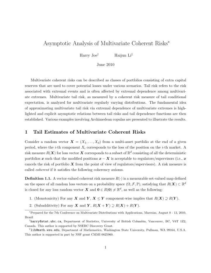
Asymptotic Analysis of Multivariate Coherent Risks ∗ Harry Joe † Haijun Li ‡ June 2010 Multivariate coherent risks can be described as classes of portfolios consisting of extra capital reserves that are used to cover potential losses under various scenarios. Tail risk refers to the risk associated with extremal events and is often affected by extremal dependence among multivari- ate extremes. Multivariate tail risk, as measured by a coherent risk measure of tail conditional expectation, is analyzed for multivariate regularly varying distributions. The fundamental idea of approximating multivariate tail risk via extremal dependence of multivariate extremes is high- lighted and explicit asymptotic relations between tail risks and tail dependence functions are then established. Various examples involving Archimedean copulas are presented to illustrate the results. 1 Tail Estimates of Multivariate Coherent Risks Consider a random vector X = ( X 1 , . . . , X d ) from a multi-asset portfolio at the end of a given period, where the i -th component X i corresponds to the loss of the position on the i -th market. A risk measure R ( X ) for loss vector X corresponds to a subset of R d consisting of all the deterministic portfolios x such that the modified positions x − X is acceptable to regulators/supervisors (i.e., x cancels the risk of portfolio X from the point of view of regulators/supervisors). A risk measure is called coherent if it satisfies the following coherency axioms. Definition 1.1. A vector-valued coherent risk measure R ( · ) is a measurable set-valued map defined on the space of all random loss vectors on a probability space (Ω , F , P ), satisfying that R ( X ) ⊂ R d is closed for any loss random vector X and 0 ∈ R ( 0 ) � = R d , as well as the following: 1. (Monotonicity) For any X and Y , X ≤ Y component-wise implies that R ( X ) ⊇ R ( Y ). 2. (Subadditivity) For any X and Y , R ( X + Y ) ⊇ R ( X ) + R ( Y ). ∗ Prepared for the 7th Conference on Multivariate Distributions with Applications, Maresias, August 8 - 13, 2010, Brazil † harry@stat.ubc.ca , Department of Statistics, University of British Columbia, Vancouver, BC, V6T 1Z2, Canada. This author is supported by NSERC Discovery Grant. ‡ lih@math.wsu.edu , Department of Mathematics, Washington State University, Pullman, WA 99164, U.S.A. This author is supported in part by NSF grant CMMI 0825960. 1
3. (Positive Homogeneity) For any X and positive s , R ( s X ) = sR ( X ). 4. (Translation Invariance) For any X and any deterministic vector l , R ( X + l ) = R ( X ) + l . The monotonicity axiom says a portfolio with more potential loss is riskier. The subadditivity is the property of risk reduction by diversification; that is, if portfolios x and y cancel the risks of X and Y respectively, then x + y cancels the risk of X + Y . The homogeneity axiom describes how portfolio size directly influences risk, whereas the translation invariance describes how incurring additional deterministic loss would affect portfolio risk. When d = 1, ̺ ( X ) := inf { r : r ∈ R ( X ) } is a univariate coherent risk measure, and thus R ( X ) = [ ̺ ( X ) , ∞ ). Univariate coherent risk measures have been extensively studied in the litera- ture [5, 8, 19], and it was shown that the popular risk measure VaR (i.e., value-at-risk), defined by VaR p ( X ) := inf { x ∈ R : Pr { X > x } ≤ 1 − p } , is not coherent and violates the subadditivity axiom. Univariate coherent risk measures can be also used to analyze risk of aggregations of multivariate portfolios, in contrast, however, the main motivation for vector-valued coherent risk measures in Definition 1.1 is that investors are sometimes not able to aggregate their multivariate portfolios on various security markets because of liquidity problems and/or transaction costs between the differ- ent security markets (e.g., having assets in several currencies at the same time, see [13] for details). The notion of vector-valued coherent risk also provides a variety of tail conditional coherent risk measures that are useful in risk allocation/decomposition for multivariate portfolios. It follows from the duality theory that any vector-valued coherent risk measure with the Fatou property (see [13]) can be expressed as follows, R ( X ) = { x ∈ R d : E Q ( x − X ) ≥ 0 , ∀ Q ∈ P} , (1.1) where P is a closed convex set of probability measures that are absolutely continuous with respect to P , and E Q ( · ) denotes the expectation with respect to Q . Clearly, R ( X ) is a convex and upper set for any loss vector X with the Fatou property. The expression (1.1) has significant practical implication and provides a scenario-based method for measuring multivariate risks; that is, P is a set of “generalized scenarios” on physical states in Ω, and R ( X ) provides the set of all deterministic portfolios of extra capitals that cover potential losses under all the scenarios specified in P . For example, if P is taken to be the set of conditional probability measures given various tail events, (1.1) yields the worst conditional expectation for random vector X , defined as W CE p ( X ) := { x ∈ R d : E ( x − X | B ) ≥ 0 , ∀ B ∈ F with P ( B ) ≥ 1 − p } , 0 < p < 1 . For any continuous random loss vector X , W CE p ( X ) equals the tail conditional expectation (TCE) for X , defined as in [6] by, { x ∈ R d : E ( x − X | X ∈ A ) ≥ 0 , ∀ A ∈ Q p ( X ) } T CE p ( X ) := � ( E ( X | X ∈ A ) + R d = + ) , 0 < p < 1 , (1.2) A ∈Q p ( X ) 2
where Q p ( X ) = { A ⊆ R d : A is upper , Pr { X ∈ A } ≥ 1 − p } . When d = 1, T CE p ( X ) = E ( X | X > VaR p ( X )) becomes the univariate coherent risk measure of tail VaR. Observe that T CE p ( X ) is a convex and upper set that consists of all the portfolios x of capital reserves that can be used to cover the expected losses E ( X | X ∈ A ) for all the tail events that X ∈ A with probability exceeding 1 − p . Tail risk can be described by W CE p ( X ) or T CE p ( X ) when p → 1. Note that multivariate coherent risk measures discussed in [13, 6] are defined for essentially bounded random vectors. To discuss asymptotic properties, these measures have to be extended to d = [ −∞ , ∞ ] d . This can be done using the idea in [8] that allows the set of all random vectors on R vectors in R ( X ) to have components taking the value of ∞ ; that is, the positions corresponding to these components are so risky, whatever that means, that no matter what the capital added, the positions will remain unacceptable. We need also to exclude the situations where components of the vectors in R ( X ) take the value of −∞ , which would mean that arbitrary amounts of capitals could be withdrawn without endangering the portfolios (see [8] for details). As a matter of fact, it can be easily verified that T CE p ( X ) is coherent in the sense of Definition 1.1 if X , which may not be bounded, has a continuous density function. The extreme value analysis of TCE T CE p ( X ) as p → 1 boils down to analyzing asymptotic behaviors of E ( X | X ∈ rB ) as r → ∞ for various upper set B , for which multivariate regular variation suits well. A non-negative random vector X with joint df F is said to have a multivariate regularly varying (MRV, see [21]) distribution F if there exists a Radon measure µ (i.e., finite on d compact sets), called the intensity measure , on R + \{ 0 } such that Pr { X ∈ rB } lim Pr {|| X || > r } = µ ( B ) , (1.3) r →∞ d + \{ 0 } 1 with µ ( ∂B ) = 0, where || · || denote a norm on R d . for any relatively compact set B ⊂ R Note that intensity measure µ ( · ) satisfies the homogeneity property that µ ( rB ) = r − α µ ( B ) for any r > 0 and any Borel-measurable set B that is bounded away from the origin. We assume that the heavy-tail index α > 1 to ensure the existence of expectations. The examples and properties of MRV distributions, including the relation between MRV distributions and multivariate extreme value distributions with identical Fr´ echet margins can be found in [21]. Since margins F 1 , . . . , F d of F are usually assumed to be tail equivalent [21], we have that the margins are regularly varying with survival function F j ( x ) = x − α L j ( x ), 1 ≤ j ≤ d , where L i ( x )’s are slowly varying [7], and L i ( x ) /L j ( x ) → c ij as x → ∞ , 0 < c ij < ∞ . We assume hereafter that c ij = 1 for notational convenience. If c ij � = 1 for some i � = j , we can properly rescale the margins and the results still follow. Observe from (1.3) that the probability of any joint tail event can be estimated proportionally by tail probabilities of the margins: for any subset B bounded away from + = [0 , ∞ ] d is compact and the punctured version R d d 1 Here R + \{ 0 } is modified via the one-point uncompactification (see, e.g., [21]). 3
Recommend
More recommend
Explore More Topics
Stay informed with curated content and fresh updates.


