3 Mixed and Continuous Strategies A pure strategy maps each of a - PDF document
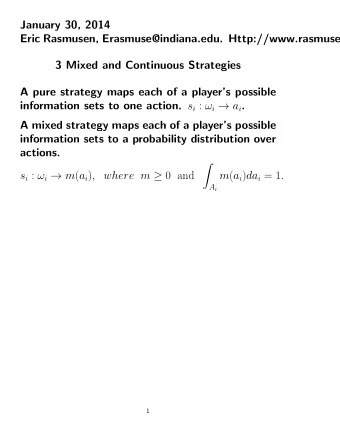
12 September 2009 Eric Rasmusen, Erasmuse@indiana.edu. Http://www.rasmusen.org 3 Mixed and Continuous Strategies A pure strategy maps each of a players possible information sets to one action. s i : i a i . A mixed strategy maps each of a
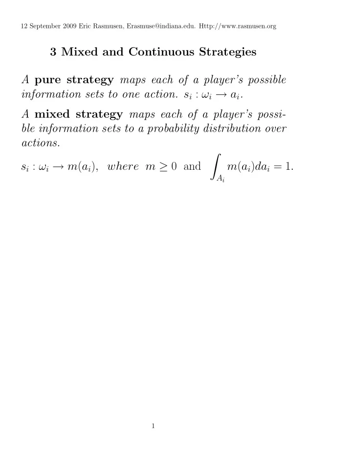
12 September 2009 Eric Rasmusen, Erasmuse@indiana.edu. Http://www.rasmusen.org 3 Mixed and Continuous Strategies A pure strategy maps each of a player’s possible information sets to one action. s i : ω i → a i . A mixed strategy maps each of a player’s possi- ble information sets to a probability distribution over actions. � s i : ω i → m ( a i ) , where m ≥ 0 and m ( a i ) da i = 1 . A i 1
Table 1: The Welfare Game Pauper Work ( γ w ) Loaf (1 − γ w ) Aid ( θ a ) 3,2 → − 1 , 3 Government ↑ ↓ No Aid (1 − θ a ) − 1 , 1 ← 0,0 Payoffs to: (Government, Pauper). Arrows show how a player can increase his payoff. If the government plays Aid with probability θ a and the pauper plays Work with probability γ w , the govern- ment’s expected payoff is π Government = θ a [3 γ w + ( − 1)(1 − γ w )] + [1 − θ a ][ − 1 γ w + 0(1 − γ w )] = θ a [3 γ w − 1 + γ w ] − γ w + θ a γ w = θ a [5 γ w − 1] − γ w . (1) Differentiate the payoff function with respect to the choice variable to obtain the first-order condition. 0 = dπ Government = 5 γ w − 1 dθ a (2) ⇒ γ w = 0 . 2 . We obtained the pauper’s strategy by differentiating the government’s payoff! 2
THE LOGIC 1 I assert that an optimal mixed strategy exists for the government. 2 If the pauper selects Work more than 20 percent of the time, the government always selects Aid . If the pauper selects Work less than 20 percent of the time, the government never selects Aid . 3 If a mixed strategy is to be optimal for the government, the pauper must therefore select Work with probability exactly 20 percent. 3
To obtain the probability of the government choosing Aid : π Pauper = γ w (2 θ a + 1[1 − θ a ]) + (1 − γ w )(3 θ a + [0][1 − θ a ]) = 2 γ w θ a + γ w − γ w θ a + 3 θ a − 3 γ w θ a = − γ w (2 θ a − 1) + 3 θ a . (3) The first-order condition is dπ Pauper = − (2 θ a − 1) = 0 , dγ w (4) ⇒ θ a = 1 / 2 . 4
The Payoff-Equating Method In equilibrium, each player is willing to mix only be- cause he is indifferent between the pure strategies he is mixing over. This gives us a better way to find mixed strategies. First, guess which strategies are being mixed between. Then, see what mixing probability for the other player makes a given player indifferent. Table 1: The Welfare Game Pauper Work ( γ w ) Loaf (1 − γ w ) Aid ( θ a ) 3,2 → − 1 , 3 Government ↑ ↓ No Aid (1 − θ a ) − 1 , 1 ← 0,0 Here, π g ( Aid ) = γ w (3)+(1 − γ w )( − 1) = π g ( No aid ) = γ w ( − 1)+(1 − γ w )(0) So γ w (3 + 1 + 1) = 1, so γ w = . 2. π p ( Work ) = θ a (2)+(1 − θ a )(1) = π p ( Loaf ) = θ a (3)+(1 − θ a )(0) so θ a (2 − 1 − 3) = − 1 and θ a = . 5. 5
Interpreting Mixed Strategies A player who selects a mixed strategy is always indif- ferent between two pure strategies and an entire contin- uum of mixed strategies. What matters is that a player’s strategy appear ran- dom to other players, not that it really be random. It could be based on time of day, temperature, etc. It could be there is a population of identical players, each of whom picks a pure strategy. But each would still be indifferent about his strategy. 6
Or, mixing could be based on unknown characteristics of the player. Harsanyi (1973). Let the payoffs not be exactly as in the matrix. In- stead, the pauper payoff of 3 is distributed on the con- tinuum [2.9, 3.1 ] with median 3. π Pauper = γ w (2 θ a + 1[1 − θ a ]) + (1 − γ w )( Xθ a + [0][1 − θ a ]) = 2 γ w θ a + γ w − γ w θ a + Xθ a − Xγ w θ a = (1 − X ) γ w θ a + (1 − X ) γ w + Xθ a . (5) The first-order condition is dπ Pauper = (1 − X ) γ w = 0 , dγ w (6) 1 ⇒ θ a = X − 1 . With probability 1, the Government has an strongly optimal pure strategy— either AID or NO AID, θ a = 1 or θ a = 0. But to the pauper, it seems there is a 50% chance of the pure strategy AID. How about if the mixing probability does not come out to .5? Well, let’s think about the government having a payoff from (Aid, Loaf) ranging from -.9 to -1.1 with cumulative distribution F ( z ). 7
π Government = θ a [3 γ w + ( z )(1 − γ w )] + [1 − θ a ][ − 1 γ w + 0(1 − γ w )] = θ a [3 γ w + z − zγ w + γ w ) − γ w = θ a [(4 + z ) γ w + z ] − γ w . (7) The first order condition tells us that the government prefers to make θ a as big as possible (that is, 1) if (4 − z ) γ w + z > 0. We need the pauper Su to think there is an unfinished 8
Table 2: Pure Strategies Dominated by a Mixed Strategy Column North South North 0,0 4,-4 Row South 4,-4 0,0 Defense 1,-1 1,-1 Payoffs to: (Row, Column) For Row, Defense is strictly dominated by (0.5 North , 0.5 South ). In equilibrium, both players choose that. His expected payoff from this mixed strategy if Col- umn plays North with probability N is 0 . 5( N )(0)+0 . 5(1 − N )(4)+0 . 5( N )(4)+0 . 5(1 − N )(0) = 2 , (8) so whatever response Column picks, Row’s expected pay- off is higher from the mixed strategy than his payoff of 1 from Defense . Lesson: It is dangerous to assume away mixed strate- gies. It is better to allow them, and then to say you will only look at pure-strategy equilibria. 9
Table 3: Chicken Jones Continue ( θ ) Swerve (1 − θ ) Continue ( θ ) − 3 , − 3 → 2, 0 Smith: ↓ ↑ Swerve (1 − θ ) 0, 2 ← 1, 1 π Jones ( Swerve ) = ( θ Smith ) · (0) + (1 − θ Smith ) · (1) = ( θ Smith ) · ( − 3) + (1 − θ Smith ) · (2) = π Jones ( Continue (9) From equation (9) we can conclude that 1 − θ Smith = 2 − 5 θ Smith , so θ Smith = 0 . 25 . In the symmetric equilibrium, both players choose the same probability, so we can replace θ Smith with simply θ . The two teenagers will survive with probability 1 − ( θ · θ ) = 0 . 9375 . 10
Jones Continue ( θ ) Swerve (1 − θ ) Continue ( θ ) − x, − x → 2, 0 Smith: ↓ ↑ Swerve (1 − θ ) 0, 2 ← 1, 1 1 θ = 1 − x. (10) If x = − 3, this yields θ = 0 . 25, as was just calculated. If x = − 9, it yields θ = 0 . 10. If x = 0 . 5, the equilibrium probability of continuing appears to be θ = 2. 11
The War of Attrition The possible actions are Exit and Continue . In each period that both Continue , each earns − 1. If a firm exits, its losses cease and the remaining firm obtains the value of the market’s monopoly profit, which we set equal to 3. We will set the discount rate equal to r > 0. (1) Continue in each period, Exit in each period (2) Each exits with probability θ if it hasn’t yet. Let Smith’s payoffs be V stay if he stays and V exit if he exits. V exit = 0. � V stay � �� V stay = θ · (3) + (1 − θ ) − 1 + , (11) 1 + r which, after a little manipulation, becomes � 1 + r � V stay = (4 θ − 1) . (12) r + θ Thus, θ = 0 . 25. 12
Timing games A pre-emption game , in which the reward goes to the player who chooses the move which ends the game, and a cost is paid if both players choose that move, but no cost is incurred in a period when neither player chooses it. Grab the Dollar . A dollar is placed on the table between Smith and Jones, who each must decide whether to grab for it or not. If both grab, each is fined one dollar. This could be set up as a one-period game, a T period game, or an infinite- period game, but the game definitely ends when someone grabs the dollar. Table 4: Grab the Dollar Jones Grab Don’t Grab Grab − 1 , − 1 → 1,0 Smith: ↓ ↑ Don’t Grab 0,1 ← 0 , 0 A noisy duel : if a player shoots and misses, the other player observes the miss and can kill the first player at his leisure. A silent duel : , a player does not know when the other player has fired, and the equilibrium is in mixed strategies. 13
Patent Race for a New Market (an all-pay auction) Players Three identical firms, Apex, Brydox, and Central. The Order of Play Each firm simultaneously chooses research spending x i ≥ 0, ( i = a, b, c ). Payoffs Firms are risk neutral and the discount rate is zero. In- novation occurs at time T ( x i ) where T ′ < 0. The value of the patent is V , and if several players innovate simul- taneously they share its value. Let us look at the payoff of firm i = a, b, c, with j and k indexing the other two firms: V − x i if T ( x i ) < Min { T ( x j , T ( x k ) } (wins) V 2 − x i if T ( x i ) = Min { T ( x j ) , T ( x k ) } ( shares with 1) < Max { T ( x j ) , T ( x k ) } π i = V 3 − x i if T ( x i ) = T ( x j = T ( x k ) (shares with 2) 2 other firms) − x i if T ( x i ) > Min { T ( x j , T ( x k ) } (loses) 14
The game Patent Race for a New Market does not have any pure strategy Nash equilibria, because the pay- off functions are discontinuous. A slight difference in research by one player can make a big difference in the payoffs, as shown in Figure 1 for fixed values of x b and x c . The research levels shown in Figure 1 are not equilibrium values. If Apex chose any research level x a less than V , Brydox would respond with x a + ε and win the patent. If Apex chose x a = V , then Brydox and Central would respond with x b = 0 and x c = 0, which would make Apex want to switch to x a = ε. 15
Figure 1: The Payoffs in Patent Race for a New Market 16
Recommend
More recommend
Explore More Topics
Stay informed with curated content and fresh updates.
