3. Correlation Options Emergence: Cross-market integration and - PowerPoint PPT Presentation
3. Correlation Options Emergence: Cross-market integration and globalization have increased the need to hedge cross-market and global positions What Are They? Correlation options are options with payoffs affected by at least two underlying
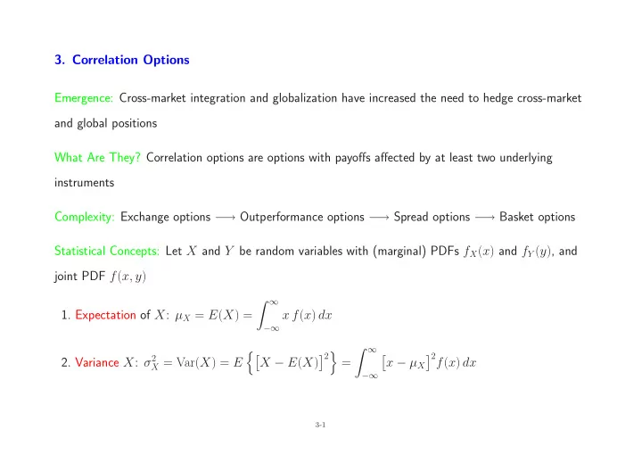
3. Correlation Options Emergence: Cross-market integration and globalization have increased the need to hedge cross-market and global positions What Are They? Correlation options are options with payoffs affected by at least two underlying instruments Complexity: Exchange options − → Outperformance options − → Spread options − → Basket options Statistical Concepts: Let X and Y be random variables with (marginal) PDFs f X ( x ) and f Y ( y ) , and joint PDF f ( x, y ) � ∞ 1. Expectation of X : µ X = E ( X ) = x f ( x ) dx −∞ � ∞ �� � 2 � � 2 f ( x ) dx 2. Variance X : σ 2 � X = Var( X ) = E X − E ( X ) = x − µ X −∞ 3-1
Statistical Concepts (continued) 3. Covariance between X and Y : � ∞ � ∞ �� �� �� � �� � σ XY = Cov( X, Y ) = E X − E ( X ) Y − E ( Y ) = x − µ X y − µ Y f ( x, y ) dx dy −∞ −∞ Cov( X, Y ) = σ XY 4. Correlation coefficient between X and Y : ρ = � � σ X σ Y Var( X ) Var( Y ) In general, Var( aX + bY ) = a 2 σ 2 X + b 2 σ 2 Y + 2 ρσ X σ Y so Var( aX + bY ) < a 2 σ 2 X + b 2 σ 2 if ρ < 0 Y Estimation of ρ : (1) Historical data (2) Implied ρ (3) Time-series analysis (e.g., GARCH model) Caution: Treating ρ as constant may be misleading and can create serious problems in risk-taking, pricing, and hedging 3-2
Historical Data: Asset price is observed at fixed intervals of time (e.g., daily, weekly, monthly) Define: n + 1 = number of observations, S j ( t i ) = j th asset price at end of i th interval, τ = length of time interval in years S 1 ( t 0 ) S 1 ( t i ) S 1 ( t n ) S 2 ( t 0 ) S 2 ( t i ) S 2 ( t n ) t 0 t 1 t 2 t 3 t 4 · · · t i · · · t n � � � � Let X ( t i ) = ln S 1 ( t i ) /S 1 ( t i − 1 ) and Y ( t i ) = ln S 2 ( t i ) /S 2 ( t i − 1 ) Assume X ( t i ) and Y ( t i ) have zero mean We estimate the standard deviation of X and of Y by � � n n � � � 1 � 1 � � � � X ( t i ) 2 Y ( t i ) 2 v X = ˆ and v Y = ˆ n n i =1 i =1 3-3
Historical Data (continued) We estimate the volatility of S 1 and of S 2 by σ 1 = ˆ v X 2 = ˆ v Y σ ∗ √ τ √ τ ˆ and ˆ We estimate the covariance between X and Y by n v XY = 1 � ˆ X ( t i ) Y ( t i ) n i =1 We estimate the correlation coefficient between X and Y (or between S 1 and S 2 ) by ρ = ˆ v XY = ˆ v XY ˆ v X ˆ ˆ v Y σ 1 ˆ ˆ σ 2 τ Generally, time should be measured by trading days so days when the exchange is closed should be ignored for volatility/correlation calculation 3-4
Price Processes: The two asset prices are assumed to be bivariate lognormally distributed Specifically, the price processes S 1 and S 2 both follow geometric Brownian motion: dS i ( t ) = ( µ i − q i ) S i ( t ) dt + σ i S i ( t ) dB i ( t ) , i = 1 , 2 where B 1 ( t ) and B 2 ( t ) are standard Brownian motions with correlation coefficient ρ In a risk-neutral world, we set µ 1 = µ 2 = r : r − q i − σ 2 �� � � i S i ( t ) = S i exp t + σ i B i ( t ) , i = 1 , 2 2 1. X ( t ) = ln[ S 1 ( t ) /S 1 ] ∼ N ( µ X , σ 2 X ) with µ X = ( r − q 1 − σ 2 σ 2 X = σ 2 1 / 2) t and 1 t 2. Y ( t ) = ln[ S 2 ( t ) /S 2 ] ∼ N ( µ Y , σ 2 Y ) with µ Y = ( r − q 2 − σ 2 σ 2 Y = σ 2 2 / 2) t and 2 t 3. X and Y jointly normally distributed with correlation coefficient ρ 3-5
Bivariate Normal Distribution: The joint PDF is − u 2 − 2 ρuv + v 2 � � 1 u = x − µ X v = y − µ Y f ( x, y ) = 1 − ρ 2 exp where and 2(1 − ρ 2 ) � σ X σ Y 2 πσ X σ Y rho = 0.5 rho = 0.9 rho = −0.9 rho = 0 3 3 3 3 2 2 2 2 0 . 0.05 0 5 0.04 0.1 0 . 1 0.06 0.08 0.15 0.2 0.2 1 1 1 1 0.1 0 . 1 2 0.3 0.3 0 . 0.14 1 6 0.35 0 . 0.18 3 5 y 0 y 0 y 0 y 0 0.25 0.14 0 1 . 2 0.25 −1 −1 −1 −1 0 . 1 0.08 0.15 0 . 0 6 0.04 −2 −2 −2 −2 0.02 0 . 0 2 −3 −3 −3 −3 −3 −2 −1 0 1 2 3 −3 −2 −1 0 1 2 3 −3 −2 −1 0 1 2 3 −3 −2 −1 0 1 2 3 x x x x 0.15 0.3 0.3 0.15 f(x,y) f(x,y) f(x,y) f(x,y) 0.10 0.10 0.2 0.2 0.05 0.05 0.1 0.1 2 2 2 2 2 2 2 2 1 1 1 1 1 1 1 1 0 0 0 0 y −2 −1 0 y −2 −1 0 y −2 −1 0 y −2 −1 0 −1 −1 −1 −1 x x x x −2 −2 −2 −2 Contours of constant density are ellipses (not invariant under rotation about its center) 3-6
Conditional Distributions: Given that Y = y , the conditional distribution of X is again normal µ X | y = µ X + ρσ X � X | Y = y ∼ N ( µ X | y , σ 2 1 − ρ 2 X | y ) where ( y − µ Y ) and σ X | y = σ X σ Y Similarly µ Y | x = µ Y + ρσ Y � Y | X = x ∼ N ( µ Y | x , σ 2 1 − ρ 2 Y | x ) where ( x − µ X ) and σ Y | x = σ Y σ X X ~ N(0,1) and Y ~ N(0,1) with rho = 0.8 Y | X = −1.5 Y | X = 0 Y | X = 1.5 3 3 3 3 0 . 0 2 2 2 2 2 0.04 0.08 0.12 1 1 1 1 0.16 0.2 0.24 0 0 0 0 v y y y 0.22 0.18 −1 −1 −1 −1 0.14 0.1 0 . 0 6 −2 −2 −2 −2 −3 −3 −3 −3 −3 −2 −1 0 1 2 3 0.00 0.02 0.04 0.06 0.08 0.00 0.05 0.10 0.15 0.20 0.25 0.00 0.02 0.04 0.06 0.08 u f(y|x) f(y|x) f(y|x) 3-7
Standardization: X and Y are jointly normally distributed with parameters ( µ X , µ Y , σ X , σ Y , ρ ) 1a. U = X − µ X ∼ N (0 , 1) and V = Y − µ Y ∼ N (0 , 1) σ X σ Y 1b. U and V are correlated since Cov( U, V ) = ρ U + V U − V 2a. Z 1 = ∼ N (0 , 1) and Z 2 = ∼ N (0 , 1) � � 2(1 + ρ ) 2(1 − ρ ) 2b. Z 1 and Z 2 are uncorrelated since Cov( Z 1 , Z 2 ) = 0 2c. Z 1 and Z 2 follow the bivariate standard normal distribution The bivariate standard normal density is − z 2 1 + z 2 n 2 ( z 1 , z 2 ) = 1 � � 2 2 π exp = n ( z 1 ) n ( z 2 ) 2 Contours of constant density are circles (invariant under rotation about its center at the origin) 3-8
Standardization (continued) X ~ N(0,1) and Y ~ N(0,2) with rho = 0.8 U ~ N(0,1) and V ~ N(0,1) with rho = 0.8 Z1 ~ N(0,1) and Z2 ~ N(0,1) with rho = 0 0.01 3 3 4 0.02 0.03 0 . 0 4 2 2 0.06 . 0 8 0 2 0.06 0 . 0 8 0.12 0 . 1 1 1 0.16 0 . 1 0.2 0.12 2 0 . 1 4 2 . 0 0.13 z2 y 0 v 0 0 0.24 0.11 0.18 0.12 −1 −1 0.14 0.09 0.08 −2 0.1 0.07 0.06 0.04 −2 −2 0.05 0.04 0.02 0.02 −4 0.01 −3 −3 −3 −2 −1 0 1 2 3 −3 −2 −1 0 1 2 3 −3 −2 −1 0 1 2 3 x u z1 Geometrically: 1. Step 1 involved rescaling along the x and y axes so that marginal distributions of U and V are standard normal (no correction to the “tilt”) 2. Step 2 involved adopting the principle axes of the ellipse as new coordinate system (thus correcting the “tilt”) and another rescaling so that Z 1 and Z 2 are standard normal 3-9
Simulation of Pairs of Correlated Normal Variables: A recipe based on our previous discussion 1. Generate independent standard normal variables Z 1 and Z 2 2. Set U = 1 and V = 1 � � � � � � � � Z 1 2(1 + ρ ) + Z 2 2(1 − ρ ) Z 1 2(1 + ρ ) − Z 2 2(1 − ρ ) 2 2 ⇒ U and V are standard normal variables with correlation ρ 3. Set X = µ X + σ X U and Y = µ Y + σ X V X ∼ N ( µ X , σ 2 X ) and Y ∼ N ( µ Y , σ 2 ⇒ Y ) with correlation ρ Multivariate Normal Distribution: Concepts developed for the bivariate normal distrbution generalized naturally to the n -variate normal distribution 1. n means [mean vector] 2. n variances and n ( n − 1) / 2 pairwise covariances/correlations [covariance/correlation matrix] 3. Contours of constant density are hyperellipsoids 3-10
Useful Property: Application of rotational invariance of the bivariate standard normal distribution If Z 1 and Z 2 follow a bivariate standard normal distribution, then � ∞ � a + bz 1 � a � √ P { Z 2 < a + bZ 1 } = n 2 ( z 1 , z 2 ) dz 2 dz 1 = N 1 + b 2 −∞ −∞ 3-11
3-1. Exchange Options Motivating Example: Exchange options embedded in DIB notes � � Redemption value = gearing × min { index 1 , index 2 } = gearing × index 1 − max { 0 , index 1 − index 2 } Embedded in the DIB note is the sale by the investor of an option to exchange index 1 for index 2 The option premium is used to increase the gearing of the note so the DIB note will pay in excess of 100% of the upside of the minimum of the two indices Example: An investor with a bullish view on both oil and gold can purchase a note with a redemption value of 107% (“gearing”) of the minimum value of 44,444 oz gold and 1,075,350 barrels oil For an investor who is bullish on both indices, this structure offers a higher expected return than a portfolio in the two indices 3-12
Recommend
More recommend
Explore More Topics
Stay informed with curated content and fresh updates.
