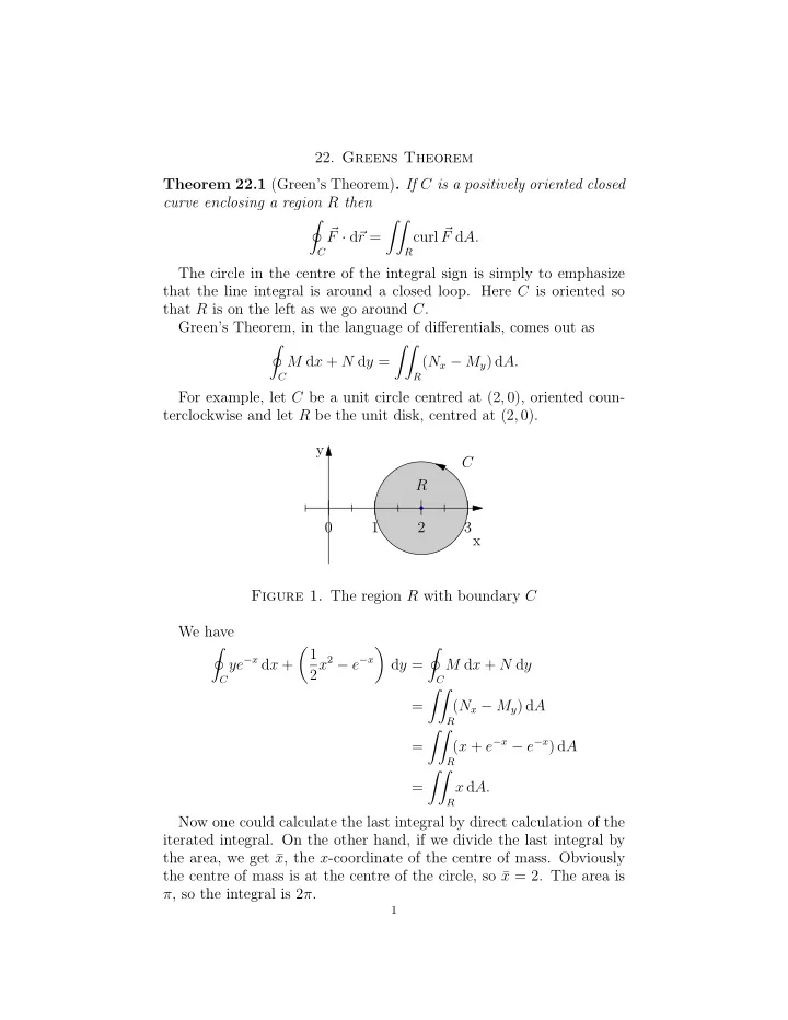
22. Greens Theorem Theorem 22.1 (Greens Theorem) . If C is a - PDF document

22. Greens Theorem Theorem 22.1 (Green’s Theorem) . If C is a positively oriented closed curve enclosing a region R then � �� � curl � F · d � r = F d A. C R The circle in the centre of the integral sign is simply to emphasize that the line integral is around a closed loop. Here C is oriented so that R is on the left as we go around C . Green’s Theorem, in the language of differentials, comes out as � �� M d x + N d y = ( N x − M y ) d A. C R For example, let C be a unit circle centred at (2 , 0), oriented coun- terclockwise and let R be the unit disk, centred at (2 , 0). y C R 0 1 2 3 x Figure 1. The region R with boundary C We have � � 1 � � ye − x d x + 2 x 2 − e − x d y = M d x + N d y C C �� = ( N x − M y ) d A R �� ( x + e − x − e − x ) d A = R �� = x d A. R Now one could calculate the last integral by direct calculation of the iterated integral. On the other hand, if we divide the last integral by the area, we get ¯ x , the x -coordinate of the centre of mass. Obviously the centre of mass is at the centre of the circle, so ¯ x = 2. The area is π , so the integral is 2 π . 1

Corollary 22.2. Let � F = M ˆ ı + N ˆ  be a vector field which is defined and differentiable on the whole of R 2 . Then � F is a gradient vector field if and only if M y = N x . Proof. Suppose that M y = N x . Then curl � F = 0. By ( ?? ), we have � �� �� � curl � F · d � r = F d A = 0 d A = 0 . C R R Hence � F is conservative. � Note that this only works if the region R is completely contained in the locus where � F is defined. In question B5 of last weeks hwk, the integral around the unit circle the vector field � F is not defined at the origin. We now describe the proof of ( ?? ) Proof of ( ?? ) . First a couple of useful reduction steps. For a start it suffices to prove two separate identities: � �� � �� M d x = − M y d A and N d y = N x d A. C R C R To get the general result, add these two identities. Secondly, if R is the union of two regions R 1 and R 2 and we know the result for both regions R 1 and R 2 then we know it for R . Indeed, � � � � � � F · d � r = F · d � r + F · d � r C C 1 C 2 �� �� curl � curl � = F d A + F d A R 1 R 2 �� curl � = F d A. R Here C is the boundary of R and C 1 , C 2 are the boundaries of R 1 and R 2 . The first equality is therefore a little bit more subtle than might first appear; the key thing is that we might get some cancelling. Using these two reduction steps, we get down to the kernel of the proof. Prove that � �� M d x = − M y d A C R where R is a vertically simple region, that is a region of the form a ≤ x ≤ b and f 0 ( x ) ≤ y ≤ f 1 ( x ) . 2

y C 3 , y = f 1 ( x ) R C 4 C 2 C 1 , y = f 0 ( x ) x a b Figure 2. Typical vertically simple region So R is the region between the graph of two functions. Now we calculate both sides. For the LHS break C into four pieces, C = C 1 + C 2 + C 3 + C 4 , where C 1 is the lower edge, the graph of y = f 0 ( x ) between a and b , C 2 is the right vertical segment, C 3 is the upper edge, the graph of y = f 1 ( x ) between a and b , and C 4 is the left vertical segment. Now � � M d x = M d x = 0 , C 2 C 4 since x is constant on these edges. For the other two edges use the parametrisation x ( t ) = t , y ( t ) = f 0 ( t ), a ≤ t ≤ b and x ( t ) = t , y ( t ) = f 1 ( t ), a ≤ t ≤ b , but with the opposite orientation, so that we get � b � b � � � M d x = M d x + M d x = M ( t, f 0 ( t )) d t − M ( t, f 1 ( t )) d t. C C 1 C 3 a a For the RHS we have � b � f 1 ( x ) �� − M y d A = − M y d y d x. f 0 ( x ) R a Now the inner integral is � f 1 ( x ) � b M y d y = − M ( x, f 1 ( x )) − M ( x, f 0 ( x )) d x, f 0 ( x ) a and so the outer integral is � b M ( x, f 0 ( x )) − M ( x, f 1 ( x )) d x, a the same as the LHS. 3

There is a similar calculation with N replacing M , horizontally sim- ple regions replacing vertically simple regions and suitable switching of x and y . � Example 22.3. The area of a region R can be evaluated using Green’s theorem. For example, �� � area( R ) = 1 d A = x d y. R C One can actually build physical devices that measure area this way. If one has a figure on a piece of paper, a planimeter can be used to find the area. Move the end of the planimeter so it traces out the curve C . At the end one can read off the area. For a linear planimeter, there is an arm AB . B is constrained to lie in the y -axis and the point A traces out the curve C . Suppose it has coordinates (0 , b ). Suppose the coordinates of A are ( x, y ). So − → AB = � x, y − b � . It follows that if � F = � b − y, x � , then � F is perpendicular to − → AB . The length of � F is a constant equal to the length m of the arm. By ( ?? ) � �� M d x + N d y = ( N x − M y ) d A C R �� 1 − ∂ ( b − y ) = d A ∂y R �� = 1d A R = area( R ) . Here we used the fact that √ m 2 − x 2 ∂ ( b − y ) = ∂ = 0 . ∂y ∂y 4