2000-02-04 Lecture 12: Vector fields Hedgehogs Warping and - PowerPoint PPT Presentation

Mats Nyl´ en February 4, 2000 Slide 1 of 29 2000-02-04 • Lecture 12: – Vector fields – Hedgehogs – Warping and displacement plots – Particle traces – LIC • Lecture 13: – Modelling algorithms – Source objects: implicit functions and glyphs – Cutting • Textbook: 6.3, (6.4), 6.5, 6.6, 6.7, 6.8, 6.9, 6.10. • Extra: Article by Cabral and Leedom. • Exercises: 6.6, 6.9, 6.11,6.14 and 6.16 VIS00

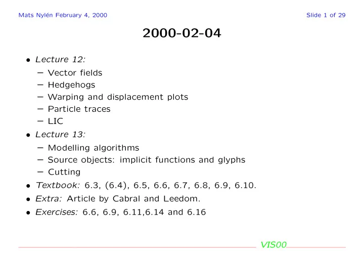
Mats Nyl´ en February 4, 2000 Slide 2 of 29 Vector fields A vector is an object with direction and length, we typically respresent a vector with it’s three Cartesian components: � V = ( V x , V y , V z ) A Vector field is a field which associates a vector with each point in space. Examples include: • Electromagnetic fields � E, � B • Flow velicities (or momentum) � v • The gradient of any scalar field � A = � ∇ T VIS00

Mats Nyl´ en February 4, 2000 Slide 3 of 29 Electromagnetic field equations These are Maxwell’s equations ∂ � � � E ∇ × � � � B = µ 0 J + ε 0 ∂t − ∂ � B ∇ × � � E = ∂t ∇ · � � E = ρ/ε 0 ∇ · � � B = 0 defining the Electric field , � E , and the Magnetic field , � B . ρ is charge density and � J is the electric current. VIS00

Mats Nyl´ en February 4, 2000 Slide 4 of 29 The Navier-Stokes equation The Navier-Stokes equation describes incompressible flow ∂� v f − 1 ∇ p + ν ∇ 2 � v · � v = � � ∂t + ( � ∇ ) � v ρ v , to an external force, � relating the flow velocity, � f , the pressure, p and the density ρ . ν is the (kinematic) viscosity. Sometimes the flow momentum , � p = ρ� v is used instead. VIS00

Mats Nyl´ en February 4, 2000 Slide 5 of 29 Steady state We call time-independent vector-fields for steady VIS00

Mats Nyl´ en February 4, 2000 Slide 6 of 29 Vector algorithms These are the basic vector algorithms: • hedgehogs • warping • particle tracing or advection algorithms • line integral convolution or LIC VIS00

Mats Nyl´ en February 4, 2000 Slide 7 of 29 Hedgehogs Draw a small directed line at some points in space VIS00

Mats Nyl´ en February 4, 2000 Slide 8 of 29 Problems with hedgehogs There are some obvious problems with hedgehogs: • visual impression depends a lot on the spatial distribution of the glyphs • using a lot of glyphs produces unwieldly pictures VIS00

Mats Nyl´ en February 4, 2000 Slide 9 of 29 Scaling of glyphs When using scaled and oriented glyphs, the impression depends a lot on the dimensionality of the glyph. This is somtimes called the “visualization lie”. VIS00

Mats Nyl´ en February 4, 2000 Slide 10 of 29 Warping Vector data which is associated with “motion” can effectively be visualised using warping . VIS00

Mats Nyl´ en February 4, 2000 Slide 11 of 29 Displacement plots We can also show displacements on a surface, plot a displacement propor- tional to s = � V · � n Where � n is the surface normal. Useful for illustrating normal modes for example VIS00

Mats Nyl´ en February 4, 2000 Slide 12 of 29 Advection for steady fields For steady fields (i.e. time- independant ) we may define field lines or stream- lines . Given a vector field � V we may define paths � r ( τ ) with the property r = � d� V dτ (where � r is a point in space). Or, as an ordinary differential equation d� r dτ = � V ( � r ) These curves forms the fieldlines or streamlines and can be used to visualize a steady field. The differential equation can be solved using standard numerical techniques, typically Runge-Kutta of order 2 or 4 is sufficient. VIS00

Mats Nyl´ en February 4, 2000 Slide 13 of 29 Tracing techniques The parametrised streamlines can be used in various ways • plot the streamlines, colour code the lines with some scalar, e.g., ve- locity, pressure etc. • plot tubes along stream, use one scalar for colour coding and another for the diameter of the tube • realease a set of particles at some initial positions and let them advect along the streamline, show this as an animation • instead of simply plotting particles, plot a glyph at the postion, this becomes a “moving” hedgehog. VIS00

Mats Nyl´ en February 4, 2000 Slide 14 of 29 Streamlines through an office This shows an example of streamlines The colours indicate pressure VIS00

Mats Nyl´ en February 4, 2000 Slide 15 of 29 Getting fancy - Streamtubes The same data but with a single streamtube, diameter of tube indicates flow-velocity. A thinner tube indicates faster flow. VIS00

Mats Nyl´ en February 4, 2000 Slide 16 of 29 Line integral convolution A slightly different idea is the line integral convolution or LIC methods. Given a vectorfield � V we generate the fieldlines that passes thorugh a given point when τ = 0 and convolve this with some texture � ∆ τ s ( � r ) = − ∆ τ T ( � r ( τ )) dτ Where T is some texture. I.e. we average a texture over a short piece of the streamline that passes through � r . Typically one uses white noise for the texture. LIC is a fairly recent invention (1993), see paper by Cabral. VIS00

Mats Nyl´ en February 4, 2000 Slide 17 of 29 A recent LIC example Visualization of flow around a car tyre VIS00

Mats Nyl´ en February 4, 2000 Slide 18 of 29 But you can also lic a flower VIS00

Mats Nyl´ en February 4, 2000 Slide 19 of 29 Tensors Tensors are 3 × 3 matrices, a general tensor is thus   t xx t xy t xz T = t yx t yy t yz     t zx t zy t zz A tensor is called symmetric if t αβ = t βα . A Tensor field is then a field which which associates a tensor with each point in space. VIS00

Mats Nyl´ en February 4, 2000 Slide 20 of 29 Tensor algorithms Below are two example tensor visualizations To the left tensor ellipsiods , to the right Hyperstreamlines VIS00

Mats Nyl´ en February 4, 2000 Slide 21 of 29 Modelling Modelling is our catch-all category of algorithms, we’ll briefly discuss some elements of modelling algorithms. VIS00

Mats Nyl´ en February 4, 2000 Slide 22 of 29 Source objects Source objects starts the visualization pipeline, inserted source objects can be classified • Modelling simple geometry, e.g. a sphere, a cone, an arrow etc. • Supporting geometry, e.g. three lines to indicate the axes or tybes wrpped around lines or supplemental input to filters such as probes or streamlines • Data attribute creation, texture data, scalar data over uniform grid. One important type of source object is an implicit function . VIS00

Mats Nyl´ en February 4, 2000 Slide 23 of 29 Implicit functions An implicit function defining a surface is f ( x, y, z ) = c this splits 3-space into 3 different domains: 1 : f ( x, y, z ) > c 2 : f ( x, y, z ) = c 3 : f ( x, y, z ) < c As an example consider a sphere modelled by x 2 + y 2 + z 2 = R 2 . We can also define operations for combining imiplicit functions. Implict functions extends to implicit modelling VIS00

Mats Nyl´ en February 4, 2000 Slide 24 of 29 More about glyphs Glyphs are very useful in visualizations of various types. A glyph is any object which is parametrised by some data • may be positioned on several points • may be scaled and rotated according to vector data • shape and colour may depend on scalar (and/or combinations of scalars and vector) • etc. VIS00

Mats Nyl´ en February 4, 2000 Slide 25 of 29 Another glyph example A face with surface normals indicated by cones VIS00

Mats Nyl´ en February 4, 2000 Slide 26 of 29 Cutting Creating cuts (like orthoslices) is a very useful visualization technique. The cuts can be generated from an implicit function F ( x, y, z ) = 0 • Generate the F ( x, y, z ) = 0 iso-surface • interpolate the attribute data (fields) onto this surface VIS00

Mats Nyl´ en February 4, 2000 Slide 27 of 29 Cutting example Yet another look at a GE cobustion chamber. The wireframe indicates the grid, colour codes the flow momentum. VIS00

Mats Nyl´ en February 4, 2000 Slide 28 of 29 Stacking cuts By stacking several semitransparent cuts we get a technique to render entire volumes VIS00

Mats Nyl´ en February 4, 2000 Slide 29 of 29 Summary and outlook With • Scalar algorithms • Vector algorithms • Modelling algorithms we are ready to start and dive into applications! One question remains: what about time-dependent data sets. VIS00