2/.5 0 0 1 2 2 Why does Fig. 1c have only - PDF document
Appeared in Proceedings of the 40th Annual Meeting of the Association for Computational Linguistics (ACL 2002) , pp. 1-8, 2002. Parameter Estimation for Probabilistic Finite-State Transducers Jason Eisner Department of Computer Science Johns
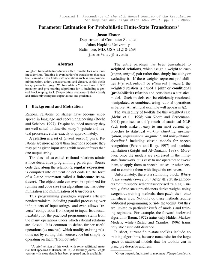
Appeared in Proceedings of the 40th Annual Meeting of the Association for Computational Linguistics (ACL 2002) , pp. 1-8, 2002. Parameter Estimation for Probabilistic Finite-State Transducers ∗ Jason Eisner Department of Computer Science Johns Hopkins University Baltimore, MD, USA 21218-2691 jason@cs.jhu.edu Abstract The entire paradigm has been generalized to weighted relations , which assign a weight to each Weighted finite-state transducers suffer from the lack of a train- ( input, output ) pair rather than simply including or ing algorithm. Training is even harder for transducers that have been assembled via finite-state operations such as composition, excluding it. If these weights represent probabili- minimization, union, concatenation, and closure, as this yields ties P ( input, output ) or P ( output | input ) , the tricky parameter tying. We formulate a “parameterized FST” weighted relation is called a joint or conditional paradigm and give training algorithms for it, including a gen- eral bookkeeping trick (“expectation semirings”) that cleanly (probabilistic) relation and constitutes a statistical and efficiently computes expectations and gradients. model. Such models can be efficiently restricted, manipulated or combined using rational operations 1 Background and Motivation as before. An artificial example will appear in § 2. The availability of toolkits for this weighted case Rational relations on strings have become wide- (Mohri et al., 1998; van Noord and Gerdemann, spread in language and speech engineering (Roche 2001) promises to unify much of statistical NLP. and Schabes, 1997). Despite bounded memory they Such tools make it easy to run most current ap- are well-suited to describe many linguistic and tex- proaches to statistical markup , chunking , normal- tual processes, either exactly or approximately. ization , segmentation , alignment , and noisy-channel A relation is a set of ( input, output ) pairs. Re- decoding , 1 including classic models for speech lations are more general than functions because they recognition (Pereira and Riley, 1997) and machine may pair a given input string with more or fewer than translation (Knight and Al-Onaizan, 1998). More- one output string. over, once the models are expressed in the finite- The class of so-called rational relations admits state framework, it is easy to use operators to tweak a nice declarative programming paradigm. Source them, to apply them to speech lattices or other sets, code describing the relation (a regular expression ) and to combine them with linguistic resources. is compiled into efficient object code (in the form Unfortunately, there is a stumbling block: Where of a 2-tape automaton called a finite-state trans- do the weights come from? After all, statistical mod- ducer ). The object code can even be optimized for els require supervised or unsupervised training. Cur- runtime and code size (via algorithms such as deter- rently, finite-state practitioners derive weights using minization and minimization of transducers). exogenous training methods, then patch them onto This programming paradigm supports efficient transducer arcs. Not only do these methods require nondeterminism, including parallel processing over additional programming outside the toolkit, but they infinite sets of input strings, and even allows “re- are limited to particular kinds of models and train- verse” computation from output to input. Its unusual ing regimens. For example, the forward-backward flexibility for the practiced programmer stems from algorithm (Baum, 1972) trains only Hidden Markov the many operations under which rational relations Models, while (Ristad and Yianilos, 1996) trains are closed. It is common to define further useful only stochastic edit distance. operations (as macros), which modify existing rela- In short, current finite-state toolkits include no tions not by editing their source code but simply by training algorithms, because none exist for the large operating on them “from outside.” space of statistical models that the toolkits can in ∗ A brief version of this work, with some additional mate- principle describe and run. rial, first appeared as (Eisner, 2001a). A leisurely journal-length 1 Given output , find input to maximize P ( input, output ) . version with more details has been prepared and is available.
b:q/.4 Abstracting away from the idea of random walks, a:p/.7 b:p/.1 arc weights need not be probabilities. Still, define a (a) (b) a: /.7 ε b:p/.03 path’s weight as the product of its arc weights and 4/.15 5/.5 b: /.03 ε b:q/.12 1/.15 the stopping weight of its final state. Thus Fig. 1a a: /.07 ε b:z/.12 b:z/.4 a:x/.63 defines a weighted relation f where f ( aabb , xz ) = b: /.1 ε . 0005292 . This particular relation does happen to be b: /.003 ε (c) q:z/1 0/.15 2/.5 b:z/.12 p:x/.9 p: /1 ε probabilistic (see § 1). It represents a joint distribu- b:x/.027 b: /.01 ε tion (since � x,y f ( x, y ) = 1 ). Meanwhile, Fig. 1c b:x/.09 p: /.1 ε 6/1 7/1 defines a conditional one ( ∀ x � y f ( x, y ) = 1 ). b:z/.4 q:z/1 3/.5 This paper explains how to adjust probability dis- tributions like that of Fig. 1a so as to model training Figure 1: (a) A probabilistic FST defining a joint probability data better. The algorithm improves an FST’s nu- distribution. (b) A smaller joint distribution. (c) A conditional distribution. Defining (a)=(b) ◦ (c) means that the weights in (a) meric weights while leaving its topology fixed. can be altered by adjusting the fewer weights in (b) and (c). How many parameters are there to adjust in Fig. 1a? That is up to the user who built it! An This paper aims to provide a remedy through a FST model with few parameters is more constrained, new paradigm, which we call parameterized finite- making optimization easier. Some possibilities: state machines . It lays out a fully general approach for training the weights of weighted rational rela- • Most simply, the algorithm can be asked to tune tions. First § 2 considers how to parameterize such the 17 numbers in Fig. 1a separately, subject to the models, so that weights are defined in terms of un- constraint that the paths retain total probability 1. A derlying parameters to be learned. § 3 asks what it more specific version of the constraint requires the means to learn these parameters from training data FST to remain Markovian : each of the 4 states must � , (what is to be optimized?), and notes the apparently present options with total probability 1 (at state 1 formidable bookkeeping involved. § 4 cuts through 15+.7+.03.+.12=1). This preserves the random-walk the difficulty with a surprisingly simple trick. Fi- interpretation and (we will show) entails no loss of nally, § 5 removes inefficiencies from the basic algo- generality. The 4 restrictions leave 13 free params. rithm, making it suitable for inclusion in an actual • But perhaps Fig. 1a was actually obtained as toolkit. Such a toolkit could greatly shorten the de- the composition of Fig. 1b–c, effectively defin- velopment cycle in natural language engineering. ing P ( input, output ) = � mid P ( input, mid ) · P ( output | mid ) . If Fig. 1b–c are required to re- 2 Transducers and Parameters main Markovian, they have 5 and 1 degrees of free- dom respectively, so now Fig. 1a has only 6 param- Finite-state machines, including finite-state au- eters total. 2 In general, composing machines mul- tomata ( FSA s) and transducers ( FST s), are a kind tiplies their arc counts but only adds their param- of labeled directed multigraph. For ease and brevity, eter counts. We wish to optimize just the few un- we explain them by example. Fig. 1a shows a proba- derlying parameters, not independently optimize the bilistic FST with input alphabet Σ = { a , b } , output many arc weights of the composed machine. alphabet ∆ = { x , z } , and all states final. It may • Perhaps Fig. 1b was itself obtained by the proba- be regarded as a device for generating a string pair in Σ ∗ × ∆ ∗ by a random walk from � � . Two paths � bilistic regular expression ( a : p ) ∗ λ ( b : ( p + µ q )) ∗ ν 0 with the 3 parameters ( λ, µ, ν ) = ( . 7 , . 2 , . 5) . With exist that generate both input aabb and output xz : ρ = . 1 from footnote 2, the composed machine � a : x /. 63 � a : ǫ/. 07 � b : ǫ/. 03 � b : z /. 4 � � � − → − → − → − → 2/.5 0 0 1 2 2 Why does Fig. 1c have only 1 degree of freedom? The Markovian requirement means something different in Fig. 1c, � a : x /. 63 � a : ǫ/. 07 � b : z /. 12 � b : ǫ/. 1 � � � − → − → − → − → 2/.5 0 0 1 2 which defines a conditional relation P ( output | mid ) rather than a joint one. A random walk on Fig. 1c chooses among arcs � with input with a given input label. So the arcs from state 6 Each of the paths has probability .0002646, so p must have total probability 1 (currently .9+.1). All other arc the probability of somehow generating the pair choices are forced by the input label and so have probability 1. ( aabb , xz ) is . 0002646 + . 0002646 = . 0005292 . The only tunable value is .1 (denote it by ρ ), with . 9 = 1 − ρ .
Recommend
More recommend
Explore More Topics
Stay informed with curated content and fresh updates.
