12 Symbolic MT 1: The IBM Models and EM Algorithm Up until now, we - PDF document

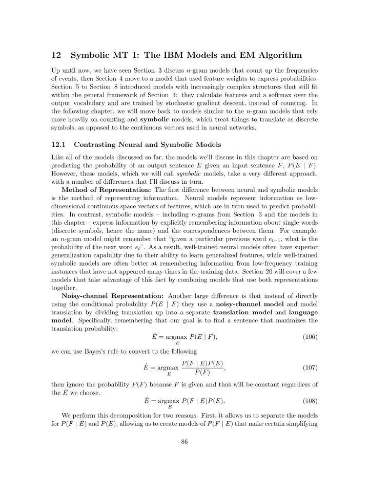
12 Symbolic MT 1: The IBM Models and EM Algorithm Up until now, we have seen Section 3 discuss n -gram models that count up the frequencies of events, then Section 4 move to a model that used feature weights to express probabilities. Section 5 to Section 8 introduced models with increasingly complex structures that still fit within the general framework of Section 4: they calculate features and a softmax over the output vocabulary and are trained by stochastic gradient descent, instead of counting. In the following chapter, we will move back to models similar to the n -gram models that rely more heavily on counting and symbolic models, which treat things to translate as discrete symbols, as opposed to the continuous vectors used in neural networks. 12.1 Contrasting Neural and Symbolic Models Like all of the models discussed so far, the models we’ll discuss in this chapter are based on predicting the probability of an output sentence E given an input sentence F , P ( E | F ). However, these models, which we will call symbolic models, take a very di ff erent approach, with a number of di ff erences that I’ll discuss in turn. Method of Representation: The first di ff erence between neural and symbolic models is the method of representing information. Neural models represent information as low- dimensional continuous-space vectors of features, which are in turn used to predict probabil- ities. In contrast, symbolic models – including n -grams from Section 3 and the models in this chapter – express information by explicitly remembering information about single words (discrete symbols, hence the name) and the correspondences between them. For example, an n -gram model might remember that “given a particular previous word e t � 1 , what is the probability of the next word e t ”. As a result, well-trained neural models often have superior generalization capability due to their ability to learn generalized features, while well-trained symbolic models are often better at remembering information from low-frequency training instances that have not appeared many times in the training data. Section 20 will cover a few models that take advantage of this fact by combining models that use both representations together. Noisy-channel Representation: Another large di ff erence is that instead of directly using the conditional probability P ( E | F ) they use a noisy-channel model and model translation by dividing translation up into a separate translation model and language model . Specifically, remembering that our goal is to find a sentence that maximizes the translation probability: ˆ E = argmax P ( E | F ) , (106) E we can use Bayes’s rule to convert to the following P ( F | E ) P ( E ) ˆ E = argmax , (107) P ( F ) E then ignore the probability P ( F ) because F is given and thus will be constant regardless of the ˆ E we choose. ˆ E = argmax P ( F | E ) P ( E ) . (108) E We perform this decomposition for two reasons. First, it allows us to separate the models for P ( F | E ) and P ( E ), allowing us to create models of P ( F | E ) that make certain simplifying 86

assumptions to make models easier (explained in a bit). The neural network models that we’ve explained before do not make these simplifying assumptions, thus sidestepping this issue. Second, it allows us to train the two models on di ff erent resources: P ( F | E ) must be trained on bilingual data, which is relatively scarce, but P ( E ) can be trained on monolingual data, which is available in large quantities. Because standard neural machine translation systems do not take this noisy channel approach, they are unable to directly use monolingual data, although there have been methods proposed to incorporate language models [8], train NMT systems by automatically translating target language data into the source language and using this as pseudo-parallel data to train the model [15], or even re-formulating neural models to follow the noisy channel framework [18]. Latent Derivations: A second di ff erence from the models in previous sections is that these symbolic models are driven by a latent derivation D that describes the process by which the translation was created. Because we don’t know which D is the correct one, we calculate the probability P ( E | F ) or P ( F | E ) by summing over these latent derivations as follows: X P ( E | F ) = P ( E, D | F ) . (109) D It is also common to approximate this value by using the derivation with the maximum probability P ( E | F ) = max D P ( E, D | F ) . (110) The neural network models also had variables that one might think of as part of a deriva- tion: the word embeddings, hidden layer states, and attention vectors. The important dis- tinction between these variables and the ones in the model above is whether they have a probabilistic interpretation (i.e. whether they are random variables or not). In the cases mentioned above, the hidden variables in neural networks do not have any probabilistic in- terpretation – given the input, the hidden variables are simply calculated deterministically, so we do not have any concept of the probability of the hidden state h given the input x , P ( h | x ). This probabilistic interpretation can be useful if we, for example, express interest in the latent representations (e.g. word alignments) and would like to calculate the probability of obtaining particular latent representations. 37 12.2 IBM Model 1 Because this is all a bit abstract, let’s go to a concrete example: IBM Model 1 [3], an example of which is shown in Figure 32. Model 1 is a model for P ( F | E ), and is extremely simple (in fact, over-simplified), in that it assumes that we first pick the number of words in the source | F | , then independently calculate the probability of each word in F . By doing so, we can assume that the probability takes the following form: | F | Y P ( F | E ) = P ( | F | | E ) P ( f j | E ) . (111) j =1 Because | F | is the length of the source sentence, which we already know, Model 1 does not make much e ff ort to estimate this length, setting the probability to a constant: P ( | F | | E ) = ✏ . 37 While not a feature of vanilla neural networks, there are ways to think about neural networks in a proba- bilistic framework, which we’ll discuss a bit more in Section 18. 87

A = 1 5 4 5 2 F = me-ri wa ke-ki wo tabeta E = mary ate a cake NULL Figure 32: An example of the variables in IBM model 1. More important is the estimation of the probability P ( f j | E ). This is done by assuming that f j was generated by the following two-step process: 1. Randomly select an alignment a j for word f j . The value of the alignment variable is an integer 1  a j  | E | + 1 corresponding to the word in E to which f j corresponds. e | E | +1 is a special NULL symbol, which is used as a catch-all token that can generate words that do not explicitly correspond to any other words in the source sentence. We assume that the alignment is generated according to a uniform distribution: P ( a j | E ) = 1 / ( | E | + 1) . (112) 2. Based on this alignment, calculate the probability of f j according to P ( f j | e a j ). This probability is a model parameter, which we learn using an algorithm described in the next section. Putting these two probabilities together, we now have the following probability for the alignments and source sentence given the target sentence: | F | Y P ( F, A | E ) = P ( | F | | E ) P ( f j | e a j ) P ( a j | E ) , (113) j =1 | F | 1 Y = ✏ | E | + 1 P ( f j | e a j ) . (114) j =1 | F | ✏ Y = P ( f j | e a j ) . (115) ( | E | + 1) | F | j =1 It should be noted that alignment A is one example of the derivation D described in the previous section. As such, according to Equation 109, we can also calculate the probability P ( E | F ) by summing over the possible alignments A : | F | ✏ X Y P ( F | E ) = P ( f j | e a j ) , (116) ( | E | + 1) | F | A j =1 | E | +1 | E | +1 | E | +1 | F | ✏ X X X Y = . . . P ( f j | e a j ) . (117) ( | E | + 1) | F | a 1 =1 a 2 =1 a | F | =1 j =1 88