10-601B Recitation 2 Calvin McCarter September 10, 2015 1 Least - PDF document

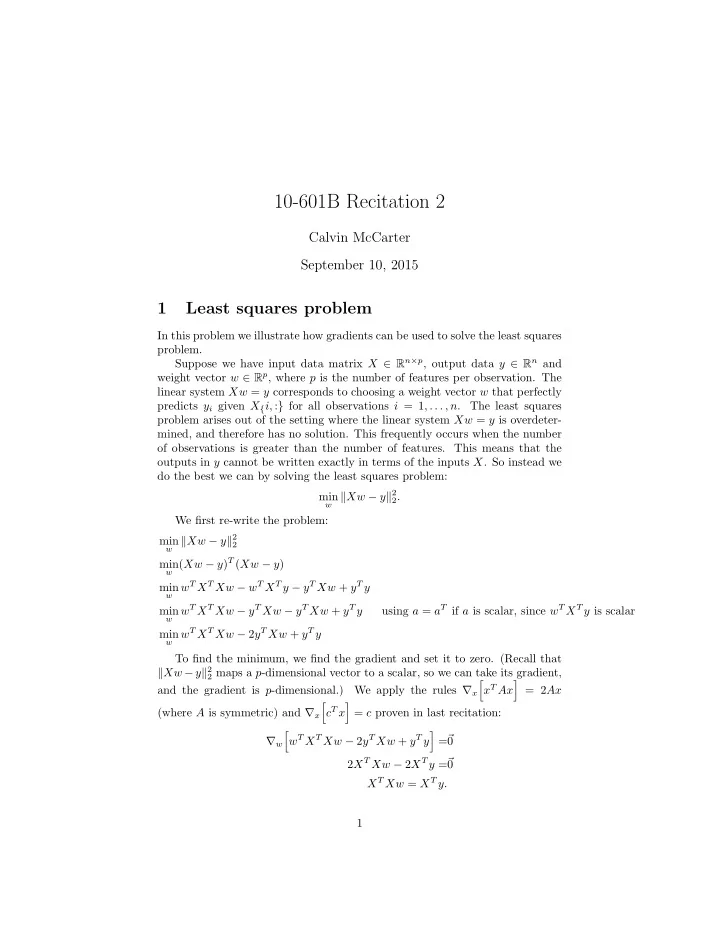
10-601B Recitation 2 Calvin McCarter September 10, 2015 1 Least squares problem In this problem we illustrate how gradients can be used to solve the least squares problem. Suppose we have input data matrix X ∈ R n × p , output data y ∈ R n and weight vector w ∈ R p , where p is the number of features per observation. The linear system Xw = y corresponds to choosing a weight vector w that perfectly predicts y i given X { i, : } for all observations i = 1 , . . . , n . The least squares problem arises out of the setting where the linear system Xw = y is overdeter- mined, and therefore has no solution. This frequently occurs when the number of observations is greater than the number of features. This means that the outputs in y cannot be written exactly in terms of the inputs X . So instead we do the best we can by solving the least squares problem: w � Xw − y � 2 min 2 . We first re-write the problem: w � Xw − y � 2 min 2 w ( Xw − y ) T ( Xw − y ) min w w T X T Xw − w T X T y − y T Xw + y T y min w w T X T Xw − y T Xw − y T Xw + y T y using a = a T if a is scalar, since w T X T y is scalar min w w T X T Xw − 2 y T Xw + y T y min To find the minimum, we find the gradient and set it to zero. (Recall that � Xw − y � 2 2 maps a p -dimensional vector to a scalar, so we can take its gradient, � � x T Ax and the gradient is p -dimensional.) We apply the rules ∇ x = 2 Ax � c T x � (where A is symmetric) and ∇ x = c proven in last recitation: � w T X T Xw − 2 y T Xw + y T y � = � ∇ w 0 2 X T Xw − 2 X T y = � 0 X T Xw = X T y. 1

Recall that X T X is just a matrix, and X T y is just a vector, so w once again is the solution to a linear system. But unlike Xw = y , which had n equations and p unknowns, here we have p equations and p unknowns, so there will be at least one solution. In the case where X T X is invertible, we have w = ( X T X ) − 1 X T y = X − 1 ( X T ) − 1 X T y = X − 1 y , so we recover the solution to Xw = y . Otherwise, we can choose any one of the infinite number of solutions, for example w = ( X T X ) + Xy , where A + denotes the pseudoinverse of A . 2 Matlab tutorial If you missed recitation and aren’t familiar with Matlab, please watch the first 27 minutes of this video: 10-601 Spring 2015 Recitation 2. Here are the commands I used 3+4 x = 3 x = 3; y = ' hello ' ; y = sprintf( ' hello world \%i \%f ' , 1, 1.5); disp(y) zeros(3,4) eye(3) ones(5) rand(2,3) A = 1+2*rand(2,3) randn(4,1) mu = 2; stddev = 3; mu + stddev*randn(4,1) size(A) numel(A) who whos clear A = rand(10,5) A(2,4) A(1:5,:) subA = A([1 2 5], [2 4]) A(:,1) = zeros(10,1); size(A(:)) X = ones(5,5); Y = eye(5); X ' inv(X) X * Y 2

X .* Y log(A) abs(A) max(X, Y) X.^2 sum(A) sum(A,1) sum(A,2) max(A,[],1) max(A,[],2) v = rand(5,2) v>0.5 v(v>0.5) index=find(v>0.5) v(index) [row_ix, col_ix] = find(v>0.5) v(row_ix,col_ix) for i=1:10 disp(i) end x = 5; if (x < 10) disp( ' hello ' ); elseif (x>10) disp( ' world ' ); else disp( ' moon ' ); end clear load( ' ecoli.mat ' ); imagesc(xTrain); plot(xTrain(:,1)); 3 MAP estimate for the Bernoulli distribution 3.1 Background The probability distribution of a Bernoulli random variable X i parameterized by µ is: p ( X i = 1; µ ) = µ and p ( X i = 0; µ ) = 1 − µ 3

We can write this more compactly (verify for yourself!): p ( X i ; µ ) = µ X i (1 − µ ) 1 − X i , X i ∈ 0 , 1 . Also, recall from lecture that for a dataset with n iid samples, we have: n � X i (1 − µ ) � � (1 − X i ) p ( X ; µ ) = p ( X 1 , . . . , X n ; µ ) = p ( X i ; µ ) = µ i =1 n � � � log p ( X ; µ ) = X i log µ + (1 − X i ) log(1 − µ ) (1) . i =1 Finally, recall that we found the MLE by taking the derivative and setting to 0: ∂µ log p ( X ; µ ) = 1 ∂ 1 � � X i − (1 − X i ) = 0 (2) 1 − µ µ � X i = # of heads ⇒ ˆ µ MLE = # of flips n 3.2 MAP estimation In the previous section µ was an unknown but fixed parameter. Now we consider µ a random variable, with a prior distribution p ( µ ) and a posterior distribution after observing the coin flips p ( µ | X ). We’re going to find the peak of the pos- terior distribution: µ MAP = argmax ˆ p ( µ | X ) µ p ( X | µ ) p ( µ ) = argmax p ( X ) µ = argmax p ( X | µ ) p ( µ ) µ = argmax log p ( X | µ ) + log p ( µ ) µ So now we find the MAP estimate by taking the derivative and setting to 0: ∂ � � log p ( X ; µ ) + log p ( µ ) = 0 ∂µ Because for log p ( X | µ ) we use Eq. (1) above, we’ll be able to use Eq. (2) for ∂ ∂µ log p ( X | µ ). For log p ( µ ) we first need to specify our prior. We use the Beta distribution: 1 B ( α, β ) µ α − 1 (1 − µ ) β − 1 p ( µ ) = 1 log p ( µ ) = B ( α, β ) + ( α − 1) log( µ ) + ( β − 1) log(1 − µ ) 4

where B ( α, β ) is a nasty function that does not depend on µ . (It just normalizes ∂ p ( µ ) so that the total probability is 1.) Now we can find ∂µ log p ( µ ): 1 ∂ � � B ( α, β ) + ( α − 1) log( µ ) + ( β − 1) log(1 − µ ) ∂µ =0 + ( α − 1) 1 1 µ + ( β − 1) 1 − µ ( − 1) = 1 1 µ ( α − 1) − 1 − µ ( β − 1) . Finally, we compute our MAP estimate: � 1 � 1 1 1 � � � � X i − (1 − X i ) + µ ( α − 1) − 1 − µ ( β − 1) = 0 µ 1 − µ 1 1 � � � � � � ( X i ) + α − 1 − (1 − X i ) + β − 1 = 0 µ 1 − µ � X i + α − 1 # of heads + α − 1 ⇒ ˆ µ MAP = n + β + α − 2 = # of flips + β + α − 2 3.3 Interpreting the Bayesian estimator One way of interpreting the MAP estimate is that we pretend we had β + α − 2 extra flips, out of which α − 1 came up heads and β − 1 came up tails. If α = β = 1, ˆ µ MAP = ˆ µ MLE . In cases like this where our prior leads us to recover the MLE, we call our prior “uninformative”. It turns out that Beta( α = 1 , β = 1) reduces to a uniform distribution over [0 , 1], which lines up with our intuition about what an unbiased prior would look like! Now suppose α = β = 10, and we flip 3 heads out of 4 flips. We have 3+9 µ MLE = 0 . 75, but ˆ ˆ µ MAP = 4+18 ≈ 0 . 55. This prior corresponds to a belief that the coin is fair. Now suppose α = β = 0 . 5, and we flip 3 heads out of 4 flips. We have µ MAP = 3 − 0 . 5 µ MLE = 0 . 75, but ˆ ˆ 4 − 0 . 5 ≈ 0 . 83. Our prior is pulling our estimate away from 1 2 ! This prior corresponds to a belief that the coin is unfair (maybe it’s a magician’s coin) but we have no idea which way it’s bent. For a fixed α, β prior, what happens as we get more samples? n →∞ ˆ lim µ MAP nµ + α − 1 = lim n + β + α − 2 n →∞ = µ In other words, the MAP estimate converges like the MLE estimate to the true µ , and the effect of our prior diminishes. 5