10-601B Recitation 1 Calvin McCarter September 3, 2015 1 - PDF document

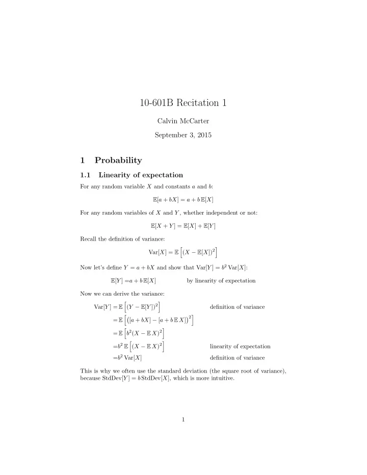
10-601B Recitation 1 Calvin McCarter September 3, 2015 1 Probability 1.1 Linearity of expectation For any random variable X and constants a and b : E [ a + bX ] = a + b E [ X ] For any random variables of X and Y , whether independent or not: E [ X + Y ] = E [ X ] + E [ Y ] Recall the definition of variance: � ( X − E [ X ]) 2 � Var[ X ] = E Now let’s define Y = a + bX and show that Var[ Y ] = b 2 Var[ X ]: E [ Y ] = a + b E [ X ] by linearity of expectation Now we can derive the variance: � ( Y − E [ Y ]) 2 � Var[ Y ] = E definition of variance �� � 2 � = E [ a + bX ] − [ a + b E X ] � b 2 ( X − E X ) 2 � = E = b 2 E � ( X − E X ) 2 � linearity of expectation = b 2 Var[ X ] definition of variance This is why we often use the standard deviation (the square root of variance), because StdDev[ Y ] = b StdDev[ X ], which is more intuitive. 1

1.2 Prediction, and expectation, and partial derivatives Suppose we want to predict a random variable Y simply using some constant c . What value of c should we choose? Here we show that E [ Y ] is a sensible choice. But first, we need to decide what a good prediction should look like. A common choice is the mean-squared error, or MSE. We punish our prediction ever more harshly the further it gets from the observed Y . � ( Y − c ) 2 � MSE = E We now show that MSE is minimized at E [ Y ]. We set it up as an optimization problem: � ( Y − c ) 2 � min E c � Y 2 − 2 E [ Y ] c + c 2 ] = min E c E [ Y 2 ] − 2 E [ Y ] c + c 2 = min c This is a quadratic function of c . We can find the minimum of this quadratic by setting its partial derivative to 0, and solving for c : ∂ � E [ Y 2 ] − 2 E [ Y ] c + c 2 � =0 ∂c − 2 E [ Y ] + 2 c =0 c = E [ Y ] This minimizes the MSE! 1.3 Sample mean and the Central Limit Theorem Suppose we have n random variables X 1 , ..., X n that are independent and iden- tically distributed (iid). Suppose we don’t know what the distribution is, but we do know their expectation and variance: E [ X i ] = µ and Var[ X i ] = σ 2 for i = 1 , ..., n A common way to estimate the unknown µ is to use the average (sample mean) of our data: n X n = 1 ¯ � X i n i =1 How does this estimate behave? We can characterize its behavior by deriving its expectation and variance. � X 1 + · · · + X n � E [ ¯ X n ] = E n = E [ X 1 ] + · · · + E [ X n ] linearity of expectation n = nµ n = µ 2

This tells us that ¯ X n is “unbiased” - its expected value is the true mean. � X 1 + · · · + X n � Var[ ¯ X n ] = Var n = 1 � � n 2 Var X 1 + · · · + X n = 1 � � Var[ X 1 ] + · · · + Var[ X n ] only because X i are iid - variance isn’t linear! n 2 n 2 ( n Var[ X i ]) = σ 2 = 1 n This tells us that the variance of the average decreases as n the number of samples increases. But it turns out we know something more about the distribution of ¯ X n . It’s distribution actually converges to a Normal distribution as n gets large. This is called the Central Limit Theorem: µ, σ 2 � � ¯ X n � N n 2 Linear Algebra I discussed problems taken directly from Section 4 of Linear Algebra Review. Two other great online resources: • YouTube tutorial on gradients • Matrix Cookbook reference 3