10.1 Active Learning Review What questions should be asked in order - PDF document

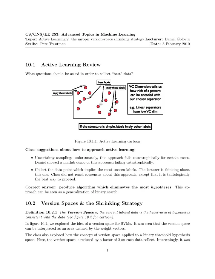
CS/CNS/EE 253: Advanced Topics in Machine Learning Topic: Active Learning 2: the myopic version-space shrinking strategy Lecturer: Daniel Golovin Scribe: Pete Trautman Date: 8 February 2010 10.1 Active Learning Review What questions should be asked in order to collect “best” data? Figure 10.1.1: Active Learning cartoon Class suggestions about how to approach active learning: • Uncertainty sampling: unfortunately, this approach fails catastrophically for certain cases. Daniel showed a matlab demo of this approach failing catastrophically. • Collect the data point which implies the most unseen labels. The lecturer is thinking about this one. Class did not reach consensus about this approach, except that it is tautologically the best way to proceed. Correct answer: produce algorithm which eliminates the most hypotheses . This ap- proach can be seen as a generalization of binary search. 10.2 Version Spaces & the Shrinking Strategy Definition 10.2.1 The Version Space of the current labeled data is the hyper-area of hypotheses consistent with the data (see figure 10.2 for cartoon). In figure 10.2, we explored the idea of a version space for SVMs. It was seen that the version space can be interpreted as an area defined by the weight vectors. The class also explored how the concept of version space applied to a binary threshold hypothesis space. Here, the version space is reduced by a factor of 2 on each data collect. Interestingly, it was 1

Figure 10.2.2: Version Space for SVMs cartoon pointed out that not any point can be collected; instead, for binary thresholds, one must choose the point closest to the middle. 1 Figure 10.2.3: Version Space for Binary threshold after successive data collects. The class then discussed an algorithm for SVMs which optimally reduced the volume of the version space. Definition 10.2.2 Suppose we are given V S ( D ) , where D is the set of labeled data. Then we define the volume of the version space: v ( x i , y i ) = vol[ V S ( D ∪ { x i , y i } )] We also define the score of the data point x i : score( x i ) = min { v ( x i , +1) , v ( x i , − 1) } 1 Indeed, in [1] an active learning algorithm produced examples for humans to classify; in almost every instance, the humans could not classify the examples. This makes sense: the most difficult examples to classify provide the most information about the true hypothesis. 2

It was then proposed that the optimal strategy is to choose x i such that score( x i ) is maximized. This approach makes intuitive sense: you want to choose the x i which has the best worst score. In other words, examine all the worst case scores for each x i —then choose the x i which does the best out of all these worst case scenarios. Mathematically, the justification for this approach is the following. Suppose each hypothesis h ∈ H is equally likely. Then E h [ v ( x i , h ( x i ))] = Pr( h ( x i ) = +1) v ( x i , +1) + Pr( h ( x i ) = − 1) v ( x i , − 1) (10.2.1) v ( x i , +1) v ( x i , − 1) = vol[ V S ( D )] v ( x i , +1) + vol[ V S ( D )] v ( x i , − 1) (10.2.2) = 1 V ( v 2 +1 ,i + v 2 − 1 ,i ) (10.2.3) where v b,i = v ( x i , b ) and V = vol[ V S ( D )] = v +1 ,i + v − 1 ,i . Since we want to shrink the space, we are interested in finding the minimum value of v 2 +1 ,i + v 2 − 1 ,i , for each x i , such that V = v +1 ,i + v − 1 ,i . This optimization is similar to the constrained optimization problem x 2 + y 2 min i subject to x + y = c whose solution is x = y = c/ 2 . If we compare this to 10.2.1, we see that the best we can ever do is to choose samples x i such that we are able to split the version space in half (let x = v +1 , y = v − 1 and c = V ); that is, we cannot outperform binary search! Of course, we are not always going to be able to recover samples x i which shrink the version space by a factor of two—this result only provides an upper bound on how quickly we can shrink the version space. As it turns out, the minimum of equation 10.2.1 is given by arg max min { v +1 ,i , v − 1 ,i } i x i which is the reason that we choose x ∗ i = arg max score( x i ) . x i A paper by Dasgupta [2] was also discussed; notably, Dasgupta points out that for constructions like in figure 10.2 (what he calls “the bad news”), adaptive learning provides no benefit, and we actually have to sample all the labels. However, Dasgupta’s main result was the following theorem, which intuitively tells us that greedy active learning is approximately as good as any other strategy for minimizing the number of col- lected labels (“the good news”): 3

Figure 10.2.4: To identify target hypotheses like L 3 , we need to see all the labels. Theorem 10.2.3 If h ∈ H is sampled uniformly at random then E h [ Q greedy ] ≤ E h [ Q ∗ ]4 log( |H| ) . If h ∈ H is sampled according to π , then 1 E h [ Q greedy ] ≤ E h [ Q ∗ ]4 log( min( π ( h ))) . A paper by Tong & Koller [3], was also mentioned. In particular, this paper considers the efficacy of maximizing the minimum margin for active collection. References [1] E.B. Baum and K. Lang. Query learning can work poorly when a human oracle is used. International Joint Conference on Neural Networks , 1992. [2] S. Dasgupta. Analysis of a greedy active learning strategy. NIPS , 2004. [3] S. Tong and D. Koller. Support vector machine active learning with applications to text clas- sification. JMLR , 2001. 4