1 Preliminaries The idea in these notes is to explain a new approach - PDF document

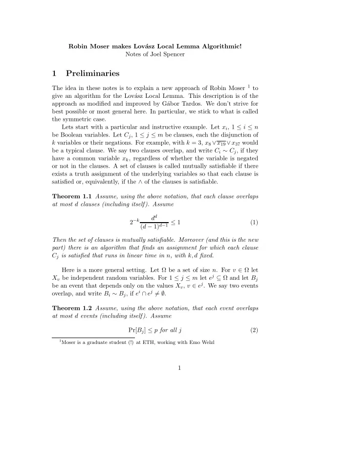
Robin Moser makes Lov´ asz Local Lemma Algorithmic! Notes of Joel Spencer 1 Preliminaries The idea in these notes is to explain a new approach of Robin Moser 1 to give an algorithm for the Lov´ asz Local Lemma. This description is of the approach as modified and improved by G´ abor Tardos. We don’t strive for best possible or most general here. In particular, we stick to what is called the symmetric case. Lets start with a particular and instructive example. Let x i , 1 ≤ i ≤ n be Boolean variables. Let C j , 1 ≤ j ≤ m be clauses, each the disjunction of k variables or their negations. For example, with k = 3, x 8 ∨ x 19 ∨ x 37 would be a typical clause. We say two clauses overlap, and write C i ∼ C j , if they have a common variable x k , regardless of whether the variable is negated or not in the clauses. A set of clauses is called mutually satisfiable if there exists a truth assignment of the underlying variables so that each clause is satisfied or, equivalently, if the ∧ of the clauses is satisfiable. Theorem 1.1 Assume, using the above notation, that each clause overlaps at most d clauses (including itself). Assume d d 2 − k ( d − 1) d − 1 ≤ 1 (1) Then the set of clauses is mutually satisfiable. Moreover (and this is the new part) there is an algorithm that finds an assignment for which each clause C j is satisfied that runs in linear time in n , with k, d fixed. Here is a more general setting. Let Ω be a set of size n . For v ∈ Ω let X v be independent random variables. For 1 ≤ j ≤ m let e j ⊆ Ω and let B j be an event that depends only on the values X v , v ∈ e j . We say two events overlap, and write B i ∼ B j , if e i ∩ e j � = ∅ . Theorem 1.2 Assume, using the above notation, that each event overlaps at most d events (including itself). Assume Pr[ B j ] ≤ p for all j (2) 1 Moser is a graduate student (!) at ETH, working with Emo Welzl 1

and that d d ( d − 1) d − 1 ≤ 1 (3) p Then ∧ m j =1 B j � = ∅ (4) Moreover (and this is the new part) there is an algorithm that finds an assignment of the X i for which each B j holds that runs in linear time in n , with k, d fixed. To say the implication of Theorem 1.1 from Theorem 1.2 consider a random assignment X v of the variables x v . That is, each X v independently takes on the values true, false with probabilities one half. The ”bad” event B j is then that the clause C j is not satisfied, which has probability 2 − k . The event that none of the bad events occur is nonempty. By Erd˝ os Magic, there is a point in the probability space, which is precisely an assignment of truth values, such that no bad event occurs, which is precisely that the clauses are all simultaneously satisfied. We will write the proof in the more general form, but the example of Theorem 1.1 is a good one to keep in mind. The time of the algorithm actually will depend on some data structure assumptions which we omit. The Moser-Tardos (ML) Algorithm . 1. Give X v random values from their distributions. 2. WHILE some B j holds. 3. PICK some B j that holds. 4. Reset the X v , v ∈ e j , independently 5. END WHILE The selection mechanism for PICK can be arbitrary. For definiteness, we may pick the minimal j for which B j holds, but it doesn’t affect the proof. We just need some specified mechanism for PICK. As this is a randomized algorithm, its output may be and will be con- sidered a random variable. Let B t , e t be the event and underlying set in the t -th iteration of the WHILE loop. We shall refer to this as time t in the running of ML. We define the LOG of the running of the algorithm to be the sequence e 1 , . . . , e t , . . . . A priori, there is no reason to believe that this algorithm will actually terminate, and so the LOG might be an infinite sequence. On the other extreme, the initial random assignment might work in which case LOG would be the null sequence. For convenience we let H = { e 1 , . . . , e m } so that the e ∈ H are just the possible values of the e t . For e ∈ H let COUNT [ e ] denote the number of times e appears in LOG, that is, the number of times t for which e = e t . A priori this could be infinite. But our main result is: 2

Theorem 1.3 1 E [ COUNT [ e ]] ≤ (5) d − 1 Given this result, linearity of expectation gives m Theorem 1.4 The expected length of LOG is at most d − 1 where m is the number of events. As each event overlaps at most d events, each v ∈ Ω can be in at most d events, and so m ≤ nd . Theorem 1.4 then gives that the expected length of LOG is linear in the size of Ω. This is why we call the MT algorithm linear time, though in particular instances one would need further assumptions about the data structure. The remainder of the argument is a proof of Theorem 1.3. Given a running of MT with the LOG of size at least t we define TREE [ t ] to be a rooted tree with vertices labelled by the e ∈ H . (Note: Several vertices may have the same label.) The root of TREE [ t ] is e t . Now we construct the tree by reverse induction from i = t − 1 to i = 1. (When t = 1 the tree has only the root e 1 .) For a given i we check whether there is a j , i < j ≤ t , such that e i , e j overlap and e j has already been placed in the tree. If there is no such j we go on to the next i , that is, we do not put e i in the tree. If there is such a j select that j for which e j is lowest (that is, furthest from the root, this part is important!) and add to the tree by making e i a child of e j . In case of ties, use an arbitrary tiebreaker, for example, pick that j with the smallest index. TREE [ t ] gives a concise description of those e i that are relevant to e t . It has certain key tautological properties. • The TREE [ t ] are all different. Reason: If s < t and TREE [ s ] , TREE [ t ] were equal, they would have to have the same root e = e s = e t . In creating TREE [ t ] each time e i = e for 1 ≤ i ≤ t there will be another node e in the tree. (When i < t as e i does overlap e t it is placed in the tree.) That is, e appears in the tree precisely the number of times in appears in e 1 , . . . , e t . When e = e s = e t , however, these numbers will be different for TREE [ s ] , TREE [ t ] as all the copies of e in TREE [ s ] are in TREE [ t ] and e t is in TREE [ t ] but not TREE [ s ]. • The e ∈ TREE [ t ] on the same level of the tree do not overlap. Reason: Suppose r < s and e r , e s ∈ TREE [ t ] and suppose they did overlap. When e r is placed in the tree it is placed as low as possible. Since e s is already in the tree it is placed on the level below e s or even lower. • When e r , e s ∈ TREE [ t ] overlap and r < s , e r is lower than e s . Reason: Above. • Let v ∈ Ω and let f 0 , . . . , f s be the nodes of TREE [ t ] that contain v . Order these by the depth of the node in the tree with the first being the furthest from the root. (From above there will be no ties.) Then the f s will be in this order in the LOG. Reason: Say 0 ≤ i < j ≤ s . After f j was placed in TREE [ t ] the later (in creating TREE ) f i overlaps f j and so is placed on the level below f j or even lower. 3