1 EXTERNAL DATA SOURCES Data Warehousing Integrated data spanning - PDF document
Data Warehousing and Decision Support [R&G] Chapter 23, Part A CS 432 1 Introduction Increasingly, organizations are analyzing current and historical data to identify useful patterns and support business strategies. Emphasis is on
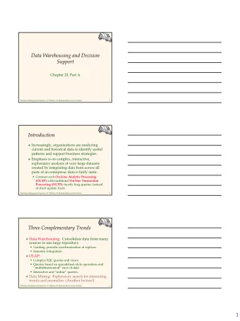
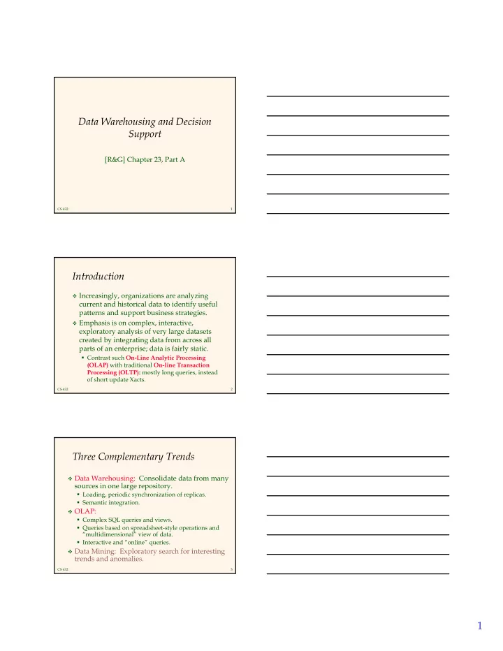
Data Warehousing and Decision Support [R&G] Chapter 23, Part A CS 432 1 Introduction � Increasingly, organizations are analyzing current and historical data to identify useful patterns and support business strategies. � Emphasis is on complex, interactive, exploratory analysis of very large datasets created by integrating data from across all parts of an enterprise; data is fairly static. � Contrast such On-Line Analytic Processing (OLAP) with traditional On-line Transaction Processing (OLTP): mostly long queries, instead of short update Xacts. CS 432 2 Three Complementary Trends � Data Warehousing: Consolidate data from many sources in one large repository. � Loading, periodic synchronization of replicas. � Semantic integration. � OLAP: � Complex SQL queries and views. � Queries based on spreadsheet-style operations and “multidimensional” view of data. � Interactive and “online” queries. � Data Mining: Exploratory search for interesting trends and anomalies. CS 432 3 1
EXTERNAL DATA SOURCES Data Warehousing � Integrated data spanning EXTRACT long time periods, often TRANSFORM LOAD augmented with summary REFRESH information. � Several gigabytes to DATA Metadata terabytes common. WAREHOUSE Repository � Interactive response times expected for SUPPORTS complex queries; ad-hoc updates uncommon. DATA OLAP MINING CS 432 4 Warehousing Issues � Semantic Integration: When getting data from multiple sources, must eliminate mismatches, e.g., different currencies, schemas. � Heterogeneous Sources: Must access data from a variety of source formats and repositories. � Replication capabilities can be exploited here. � Load, Refresh, Purge: Must load data, periodically refresh it, and purge too-old data. � Metadata Management: Must keep track of source, loading time, and other information for all data in the warehouse. CS 432 5 timeid Multidimensional locid sales pid Data Model 11 1 1 25 � Collection of numeric measures, 11 2 1 8 which depend on a set of dimensions. 11 3 1 15 � E.g., measure Sales , dimensions 12 1 1 30 Product (key: pid), Location (locid), and Time (timeid). 12 2 1 20 12 3 1 50 11 12 13 8 10 10 Slice locid=1 13 1 1 8 pid is shown: 30 20 50 13 2 1 10 25 8 15 locid 13 3 1 10 1 2 3 11 1 2 35 timeid CS 432 6 2
MOLAP vs ROLAP � Multidimensional data can be stored physically in a (disk-resident, persistent) array; called MOLAP systems. Alternatively, can store as a relation; called ROLAP systems. � The main relation, which relates dimensions to a measure, is called the fact table. Each dimension can have additional attributes and an associated dimension table. � E.g., Products(pid, pname, category, price) � Fact tables are much larger than dimensional tables. CS 432 7 Dimension Hierarchies � For each dimension, the set of values can be organized in a hierarchy: PRODUCT TIME LOCATION year quarter country category week month state pname date city CS 432 8 OLAP Queries � Influenced by SQL and by spreadsheets. � A common operation is to aggregate a measure over one or more dimensions. � Find total sales. � Find total sales for each city, or for each state. � Find top five products ranked by total sales. � Roll-up: Aggregating at different levels of a dimension hierarchy. � E.g., Given total sales by city, we can roll-up to get sales by state. CS 432 9 3
OLAP Queries � Drill-down: The inverse of roll-up. � E.g., Given total sales by state, can drill-down to get total sales by city. � E.g., Can also drill-down on different dimension to get total sales by product for each state. � Pivoting: Aggregation on selected dimensions. � E.g., Pivoting on Location and Time WI CA Total yields this cross-tabulation : 63 81 144 1995 38 107 145 � Slicing and Dicing: Equality 1996 and range selections on one 75 35 110 1997 or more dimensions. 176 223 339 Total CS 432 10 Comparison with SQL Queries � The cross-tabulation obtained by pivoting can also be computed using a collection of SQLqueries: SELECT SUM (S.sales) FROM Sales S, Times T, Locations L WHERE S.timeid=T.timeid AND S.timeid=L.timeid GROUP BY T.year, L.state SELECT SUM (S.sales) SELECT SUM (S.sales) FROM Sales S, Times T FROM Sales S, Location L WHERE S.timeid=T.timeid WHERE S.timeid=L.timeid GROUP BY T.year GROUP BY L.state CS 432 11 The CUBE Operator � Generalizing the previous example, if there are k dimensions, we have 2^k possible SQL GROUP BY queries that can be generated through pivoting on a subset of dimensions. � CUBE pid, locid, timeid BY SUM Sales � Equivalent to rolling up Sales on all eight subsets of the set {pid, locid, timeid}; each roll-up corresponds to an SQL query of the form: SELECT SUM (S.sales) Lots of work on optimizing FROM Sales S the CUBE operator! GROUP BY grouping-list CS 432 12 4
Design Issues TIMES timeid date week month quarter year holiday_flag (Fact table) pid timeid locid sales SALES PRODUCTS LOCATIONS pid pname category price locid city state country � Fact table in BCNF; dimension tables un-normalized. � Dimension tables are small; updates/inserts/deletes are rare. So, anomalies less important than query performance. � This kind of schema is very common in OLAP applications, and is called a star schema; computing the join of all these relations is called a star join. CS 432 13 Implementation Issues � New indexing techniques: Bitmap indexes, Join indexes, array representations, compression, precomputation of aggregations, etc. � E.g., Bitmap index: sex custid name sex rating rating Bit-vector: F M 1 bit for each 112 Joe M 3 10 00100 possible value. 115 Ram M 5 10 00001 Many queries can 01 119 Sue F 5 00001 be answered using bit-vector ops! 10 112 Woo M 4 00010 CS 432 14 Join Indexes � Consider the join of Sales, Products, Times, and Locations, possibly with additional selection conditions (e.g., country=“USA”). � A join index can be constructed to speed up such joins. The index contains [s,p,t,l] if there are tuples (with sid) s in Sales, p in Products, t in Times and l in Locations that satisfy the join (and selection) conditions. � Problem: Number of join indexes can grow rapidly. � A variation addresses this problem: For each column with an additional selection (e.g., country), build an index with [c,s] in it if a dimension table tuple with value c in the selection column joins with a Sales tuple with sid s; if indexes are bitmaps, called bitmapped join index. CS 432 15 5
Bitmapped Join Index TIMES timei dat week mont quarte year holiday_fla d e h r g (Fact table) pid timeid locid sales SALES PRODUCTS LOCATIONS pid pname category price locid city state country � Consider a query with conditions price=10 and country=“USA”. Suppose tuple (with sid) s in Sales joins with a tuple p with price=10 and a tuple l with country =“USA”. There are two join indexes; one containing [10,s] and the other [USA,s]. � Intersecting these indexes tells us which tuples in Sales are in the join and satisfy the given selection. CS 432 16 Querying Sequences in SQL:1999 � Trend analysis is difficult to do in SQL-92: � Find the % change in monthly sales � Find the top 5 product by total sales � Find the trailing n -day moving average of sales � The first two queries can be expressed with difficulty, but the third cannot even be expressed in SQL-92 if n is a parameter of the query. � The WINDOW clause in SQL:1999 allows us to write such queries over a table viewed as a sequence (implicitly, based on user-specified sort keys) CS 432 17 The WINDOW Clause SELECT L.state, T.month, AVG(S.sales) OVER W AS movavg FROM Sales S, Times T, Locations L WHERE S.timeid=T.timeid AND S.locid=L.locid WINDOW W AS (PARTITION BY L.state ORDER BY T.month RANGE BETWEEN INTERVAL `1’ MONTH PRECEDING AND INTERVAL `1’ MONTH FOLLOWING) Let the result of the FROM and WHERE clauses be “Temp”. � (Conceptually) Temp is partitioned according to the PARTITION BY clause. � � Similar to GROUP BY, but the answer has one row for each row in a partition, not one row per partition! Each partition is sorted according to the ORDER BY clause. � For each row in a partition, the WINDOW clause creates a “window” of � nearby (preceding or succeeding) tuples. � Can be value-based, as in example, using RANGE � Can be based on number of rows to include in the window, using ROWS clause The aggregate function is evaluated for each row in the partition using the � corresponding window. � New aggregate functions that are useful with windowing include RANK (position of a row within its partition) and its variants DENSE_RANK, PERCENT_RANK, CUME_DIST. CS 432 18 6
Recommend
More recommend
Explore More Topics
Stay informed with curated content and fresh updates.
