1 Hardy-Weinberg Principle Assumptions of Hardy Weinberg For two - PDF document
The scope of Population Genetics Why are the patterns of variation as they are? (mathematical theory) What are the forces that influence levels of variation? What is the genetic basis for evolutionary change? What data can be
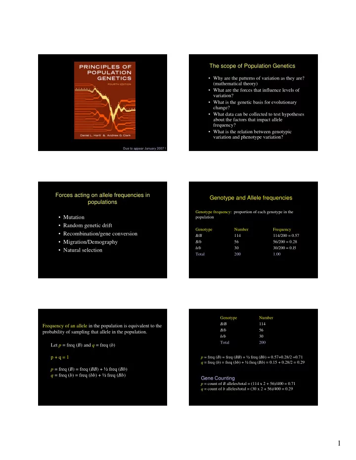
The scope of Population Genetics • Why are the patterns of variation as they are? (mathematical theory) • What are the forces that influence levels of variation? • What is the genetic basis for evolutionary change? • What data can be collected to test hypotheses about the factors that impact allele frequency? • What is the relation between genotypic variation and phenotype variation? Due to appear January 2007 ! Forces acting on allele frequencies in Genotype and Allele frequencies populations Genotype frequency: proportion of each genotype in the • Mutation population • Random genetic drift Genotype Number Frequency • Recombination/gene conversion B/B 114 114/200 = 0.57 • Migration/Demography B/b 56 56/200 = 0.28 b/b 30 30/200 = 0.l5 • Natural selection Total 200 1.00 Genotype Number B/B 114 Frequency of an allele in the population is equivalent to the B/b 56 probability of sampling that allele in the population. b/b 30 Total 200 Let p = freq ( B ) and q = freq ( b ) p + q = 1 p = freq ( B ) = freq ( BB ) + ½ freq ( Bb ) = 0.57+0.28/2 =0.71 q = freq ( b ) = freq ( bb ) + ½ freq ( Bb ) = 0.15 + 0.28/2 = 0.29 p = freq ( B ) = freq ( BB ) + ½ freq ( Bb ) q = freq ( b ) = freq ( bb ) + ½ freq ( Bb ) Gene Counting p = count of B alleles/total = (114 x 2 + 56)/400 = 0.71 q = count of b alleles/total = (30 x 2 + 56)/400 = 0.29 1
Hardy-Weinberg Principle Assumptions of Hardy Weinberg For two alleles of an autosomal gene, B and b , the •Approximately random mating genotype frequencies after one generation •An infinitely large population freq( B ) = p freq( b ) = q •No mutation freq ( B/B ) = p 2 •No migration into or out of the population freq ( B/b ) = 2 pq •No selection, with all genotypes equally viable and freq ( b/b ) = q 2 equally fertile Gene frequencies of offspring can be predicted from allele frequencies in parental generation SNPs in the ApoAI/CIII/AIV/AV region of chromosome 11 Graphical proof of Hardy Weinberg Principle Sperm B Freq of alleles in b offspring freq ( B ) = p 2 + ½ (2 pq ) B pq p 2 = p ( p + q ) = p (1) = p Eggs freq ( b ) = b q 2 q 2 + ½ (2 pq ) pq = q ( p + q ) = q (1) = q Example from MN blood typing Hardy-Weinberg tests for Quality Control MM M/N N/N Total Num. Individuals 1787 3037 1305 6129 Number M alleles 3574 3037 0 6611 Number N alleles 0 3037 2610 5647 0.5 Number M+N 3574 6074 2610 12258 Allele freq of M = 6611/12,258 = 0.53932 = p 0.4 Allele freq of N = 5647/12,258 = 0.46068 = q ObsHet p 2 = 0.29087 q 2 = 0.21222 0.3 Expected freq 2pq=0.49691 1.00 Expected # 1782.7 3045.6 1300.7 6129 0.2 (freq x 6129) χ 2 = ∑ (observed number – expected number) 2 0.1 expected number χ 2 = (1787 – 1782.7) 2 + (3037 – 3045.6) 2 + (1305 – 1300.7) 2 = 0.04887 0.0 1782.7 3045.6 1300.7 Df = number of classes of data (3) – number of parameters estimated (1) –1 = 1 df 0.0 0.5 1.0 AlleleFreq Probability of a chi-square this big or bigger = .90 Heterozygotes are being under-called (Boerwinkle et al.) 2
Hardy-Weinberg tests on steroids – the Affy 500k chip Extensions of the Hardy-Weinberg Principle • More than two alleles • More than one locus • X-chromosome • Subdivided population HW deviation = observed – expected heterozygosity CARDIA STUDY Locations of Chromosome 11 SNPs Genotyped in the AV/AIV/CIII/AI Gene Cluster (colored sites in both studies) ApoAV 124/80 † Mutation 27376 27450 27565 27673 27690 27709 27741 27820 28301 28631 28837 28943 28975 29009 29085 29590 29928 30603 30648 30730 30763 30862 30966 23/16 ApoAIV • What is the pattern of nucleotide changes? • Is the pattern of mutations homogeneous 14953 15239 15289 15423 15830 15940 15941 16081 16131 16199 16481 16600 16736 16742 16751 16845 16960 16970 17001 17366 17528 17619 17660 17766 17814 24/19 across the genome? ApoCIII • Are sites within a gene undergoing * 05406 05631 05662 05904 06156 06322 06355 06524 06723 06940 06949 06957 07073 07135 07179 07398 07446 07463 07622 07627 07761 07880 08072 08080 08143 08174 08436 08511 08519 08521 08680 08808 09102 09127 09154 09297 09301 09312 09502 09615 09616 09648 09851 09901 09907 09960 46/26 recurrent mutation? ApoAI 00523 00598 00637 00887 01046 01085 01280 01564 01616 01717 01787 01899 01962 02110 02954 02957 03132 03253 03581 03613 03710 03732 03784 03789 03923 04022 04202 04281 04699 04797 05124 31/19 Average Distance between SNPs (Fullerton 124) Average Distance between SNPs (CARDIA 80) This site is NOT included in AV AIV CIII AI ALL AV AIV CIII AI ALL Fullerton 124 † # Fullerton / # CARDIA Mean 163.18 124.39 101.20 153.37 130.05 Mean 239.33 143.06 162.24 255.61 195.03 * This part of the exon is not Std 183.83 114.98 88.77 166.32 136.83 Std 285.32 123.14 140.39 210.34 193.00 translated Observed and expected numbers of segregating sites Mutation and Random Genetic Drift (Lipoprotein lipase, LPL) • The primary parameter for drift is N e . observed expected • Mutation adds variation to the population, and drift eliminates it. • These two processes come to a steady state in which the standing level of variation is essentially constant. 3
Migration and Population Nucleotide site frequency spectrum Structure ( LPL ) • Does the Hardy-Weinberg principle hold for a population that is subdivided geographically? • What is the relation between SNP frequency, age of the mutation, and population structure? • Given data on genetic variation, how can we quantify the degree of population structure? Population heterogeneity in Jackson North Karelia 14 30 haplotype frequencies ( ApoE ) 1 17 20 1 18 4 4 28 19 23 7 2 7 2 6 Jackson 25 12 5 3 8 3 13 10 16 10 27 9 Mayan Campeche Rochester 21 26 1 4 1 4 Finland 29 11 7 2 6 7 2 15 12 5 5 3 8 3 13 31 10 16 24 Rochester 9 22 Angiotensin Converting Enzyme (ACE) Quantifying population structure Variable sites (78) • Suppose there are two subpopulations, with Individual (11) allele frequencies ( p 1 , q 1 ) and ( p 2 , q 2 ) and average allele frequencies ( P and Q ). • H T = 2 PQ = heterozygosity in one large panmictic population • H S = (2 p 1 q 1 +2 p 2 q 2 )/2 is average heterozygosity across populations • F ST = (H T -H S )/H T AA, Aa, aa Rieder et al. (1999) Note – unequal sample sizes require more calculation 4
Average F ST for human SNPs is 0.08 Population differentiation ( F ST ) Varies among SNPs and genes 0.5 0.5 0.45 0.4 0.35 0.3 F ST NR 0.25 JNR 0.2 0.15 0.1 0.05 0 0 o 4 8 2 6 0 4 8 2 6 0 4 8 2 6 0 4 8 2 6 0 4 8 2 6 0 4 8 2 N 1 1 2 2 2 3 3 4 4 4 5 5 6 6 6 7 7 8 8 8 9 9 0 0 0 1 S . 1 1 1 1 A1 C3 A4 Figure 2 Pritchard et al. method for inferring Rosenberg NA, Pritchard JK, Weber JL, Cann HM, Kidd KK, Zhivotovsky LA, Feldman MW. 2002 population substructure Genetic structure of human populations. Science. 298:2381-2385. • Specific number of subdivisions. • Randomly assign individuals. • Assess fit to HW. • Pick an individual and consider a swap. • If fit improves, accept swap, otherwise accept with a certain probability. • Markov chain Monte Carlo – gets best fitting assignment. The human mitochondrial genome – 16,659 bp European Inference of K www.mitomap.org 5
Fine-structure mapping of mitochondrial defects Major human migrations inferred from mtDNA sequences MELAS: mitochondrial myopathy encephalomyopathy lactic acidosis and stroke Genome-wide SNP discovery Ssaha SNP A C ATGCTGACTGACAT G CTAGCTGA • S equence S earch and A lignment by H ashing A lgorithm. G ATGCTGACTGACAT T CTA • Align reads; apply ad hoc filters to call SNPs ATGCTGACTGACAT T CTAG • http://www.sanger.ac.uk/Software/analysis/S TGCTGACTGACAT G CTAGC SAHA/ TGCTGACTGACAT G CTAGCT GCTGACTGACAT T CTAGCT CTGACTGACAT G CTAGCTGA Distribution of SNP Density Across the Genome Observed SNP Distribution is not Poisson λ − λ x e = Pr( x . SNPs ) x ! 6
Celera SNPs and Celera - PFP SNPs Similar inference from Celera-only as from Celera vs. public SNPs Why the Poisson distribution fits badly • Time to common ancestry for a random pair of alleles is distributed exponentially. Celera SNPs Celera - PFP • So the Poisson parameter varies from one region to another. • Because the time to common ancestry varies widely, the expected number of segregating mutations varies widely as well. • But variation in ancestry time is not sufficient to explain the magnitude of variation in SNP density. Mixture models allowing heterogeneity in mutation and recombination can fit the data well Nucleotide diversity ( x 10 -4 ) by chromosome 1 7.29 13 7.75 2 7.39 14 7.32 3 7.46 15 7.84 4 7.84 16 8.85 5 7.42 17 7.92 6 7.83 18 7.76 7 8.03 19 9.04 8 8.06 20 7.69 9 8.14 21 8.54 10 8.26 22 8.19 11 7.89 X 4.89 12 7.55 Y 2.82 Sainudiin et al, submitted Motivation Mutation-drift balance: the null model • Are genome-wide data on human SNPs •Model with pure mutation compatible with any particular MODEL? •The Wright-Fisher model of drift • Perhaps more useful -- are there models that can be REJECTED ? •Infinite alleles model • Models tell us not only about what genetic •Infinite sites model attributes we need to consider, they also •The neutral coalescent can provide quantitative estimates for rates of mutation, effective population size, etc. 7
Recommend
More recommend
Explore More Topics
Stay informed with curated content and fresh updates.
