1 Data-dr Data-driven philosophy n philosophy Data-dr - PDF document

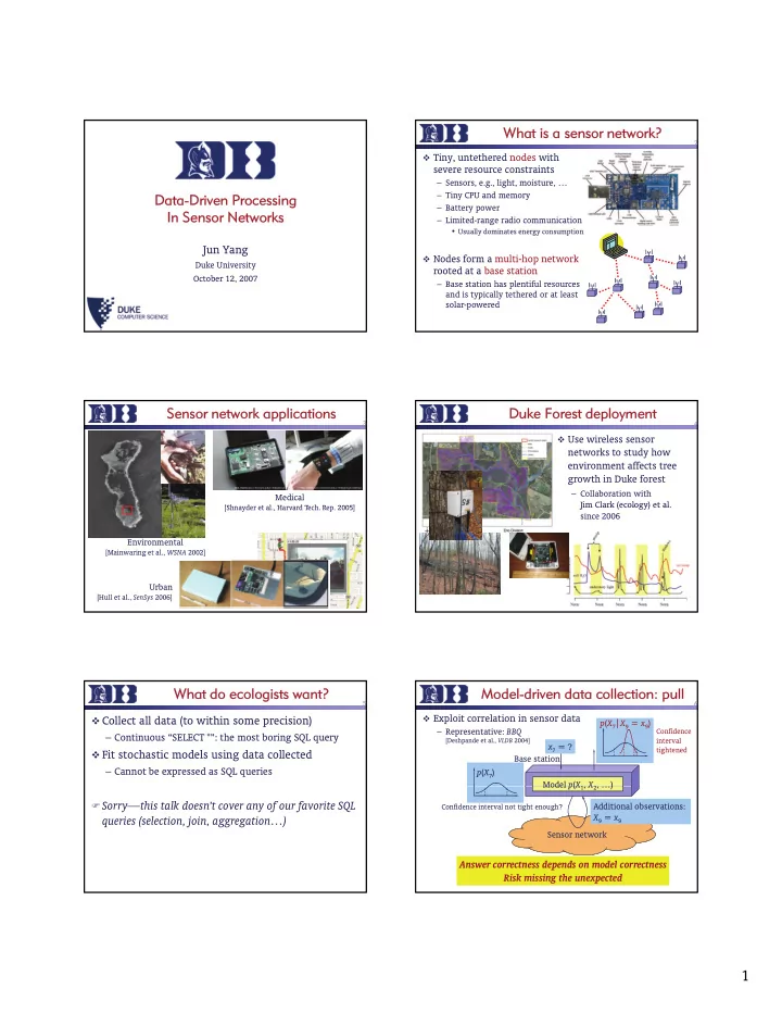
What What is is a a senso sensor network? network? 2 � Tiny, untethered nodes with severe resource constraints – Sensors, e.g., light, moisture, … – Tiny CPU and memory Da Data ta-Driven Pr -Driven Proc ocessing essing – Battery power In Sensor Networks In Sensor Networks – Limited-range radio communication • Usually dominates energy consumption Jun Yang � Nodes form a multi-hop network Duke University rooted at a base station October 12, 2007 – Base station has plentiful resources and is typically tethered or at least solar-powered Senso Sensor network network applicati applications ns Duke Forest Duke Forest deployment deployment 3 4 � Use wireless sensor networks to study how environment affects tree growth in Duke forest – Collaboration with Medical Jim Clark (ecology) et al. Jim Clark (ecology) et al [Shna der et al Har ard Tech Rep 2005] [Shnayder et al., Harvard Tech. Rep. 2005] since 2006 Environmental [Mainwaring et al., WSNA 2002] Urban [Hull et al., SenSys 2006] What do What do ecolog ecologis ists want? want? Model Model-dri rive ven data collect n data collectio ion: n: pull pull 5 6 � Exploit correlation in sensor data � Collect all data (to within some precision) p ( X 7 | X 9 = x 9 ) – Representative: BBQ Confidence – Continuous “SELECT *”: the most boring SQL query [Deshpande et al., VLDB 2004] interval x 7 = ? tightened � Fit stochastic models using data collected Base station – Cannot be expressed as SQL queries p ( X 7 ) Model p ( X 1 , X 2 , …) Model p ( X 1 , X 2 , …) � Sorry—this talk doesn’t cover any of our favorite SQL Additional observations: Confidence interval not tight enough? X 9 = x 9 queries (selection, join, aggregation…) Sensor network Answer correctness depends on model correctness Risk missing the unexpected 1

Data-dr Data-driven philosophy n philosophy Data-dr Data-driven: push n: push 7 8 � Models don’t substitute for actual readings � Exploit correlation in data + put smarts in network – Representatives: Ken [Chu et al., ICDE 2006] , Conch [Silberstein et al., – Correctness of “SELECT *” should not depend on ICDE 2006, SIGMOD 2006] correctness of models Values transmitted at time t – 1 – Particularly when we are still learning about the Base station Model p ( X ( t ) | o ( t – 1) , o ( t – 2) , …) physical process being monitored Transmit o ( t ) such that � Models can still be used to optimize “SELECT *” k x ( t ) – E( X ( t ) | o ( t ) , o ( t – 1) , …) k · ε Compare actual reading x ( t ) with model prediction Sensor network Sensor network E( X ( t ) | o ( t – 1) , o ( t – 2) , …) Model p ( X ( t ) | o ( t – 1) , o ( t – 2) , …) Differ by more than ε ? Regardless of model quality, base station knows x ( t ) to within ε Better model ⇒ fewer transmissions Tempora Temporal suppression example suppression example Spatial suppre Spatia suppression examp example 9 10 10 � Suppress transmission if � “Leader” nodes report for cluster |current reading – last transmitted reading| · ε � Others suppress if – Model: X ( t ) = x ( t – 1) |my reading – leader’s reading| · ε � Effective when readings change slowly – Model: X me = x leader � What about large-scale changes? � Effective when nearby readings are similar 10 30 10 30 30 10 20 10 30 10 30 20 10 30 10 10 Cluster 2 20 30 20 30 leader 10 30 10 30 10 10 10 20 30 30 30 10 20 30 10 20 30 10 20 30 leader 10 30 10 30 Cluster 1 10 leader 10 30 10 30 20 10 20 30 10 20 30 10 30 30 20 10 30 30 10 Cluster 3 Phenomenon is simple to describe, but all nodes transmit! Leaders always transmit! Combining spatial Combini g spatial and and temporal temporal Outline Outli ne 11 11 12 12 Spatiotemporal suppression condition = ? � Temporal AND spatial? � How to combine temporal and spatial – I.e., suppress if both suppression conditions are met suppressions effectively – Results in less suppression than either! – Conch [Silberstein et al., SIGMOD 2006] � Temporal OR spatial? p p – I.e., suppress if either suppression condition is met � What to do about —the dirty little secret – Base station cannot decide whether to set suppressed of suppression value to the previous value (temporal) or to the nearby value (spatial)! – BaySail [Silberstein et al., VLDB 2007] 2

Conch Conch = con = constra straint ch t chaini aining ng Recov Recovering ring readi reading ngs in in Conch Conch 13 13 14 14 Temporally monitor spatial constraints (edges) � Base station “chains” monitored edges to recover readings � x i and x j change in similar ways ⇒ x + ∆ 1 x + ∆ 1 + ∆ 2 + ∆ 3 temporally monitor edge difference ( x i – x j ) ∆ 1 ∆ 4 ∆ 2 – “Difference” can be generalized x ∆ 3 x + ∆ 1 + ∆ 2 + ∆ 3 + ∆ 4 x + ∆ 1 + ∆ 2 � One node is reporter and p Ch i i Chaining starting point; t ti i t the other updater ( x i – x j ) temporally monitored updates – Reporter tracks ( x i – x j ) and i reporter � Discretize values to avoid error stacking transmits it to base station j x j updates – [ k ε , k ε + ε ) → k if its value changes updater – Monitor discretized values exactly – Updater transmits its value updates to reporter • Discretization is the only source of error • I.e., temporally monitor remote input to the spatial constraint • No error introduced by suppression Conch examp Conch example Choosing what to Choosi g what to monitor monitor 15 15 16 16 � A spanning forest is necessary and sufficient to recover 0 10 30 10 0 10 20 30 30 all readings 10 30 20 0 0 0 – Each edge is a temporally monitored spatial constraint 10 30 10 10 20 30 30 Temporally monitored 0 – Each tree root is temporally monitored 0 10 20 30 start of chain 0 10 30 0 • Start of chain 0 10 10 30 20 10 30 30 20 0 0 (For better reliability, more edges can be monitored at extra cost) (For better reliability more edges can be monitored at extra cost) –20 20 10 10 30 30 10 � Some intuition Only “border” edges transmit to base station Combines advantages of both temporal and spatial suppression – Choose edges between correlated nodes – Do not connect erratic nodes • Monitor them as singleton trees in the forest Cost- Cost-based fores forest const construct uction Wave Wavefr front exp experi riment 17 17 18 18 � Simulate periodic vertical wavefronts moving across field, � Observe where sensors are randomly – In pilot phase, use any spanning forest to collect data placed at grid points • Even a poor spanning forest correctly collects all data � Optimize – Use collected data to assign monitoring costs Use collected data to assign monitoring costs Conch beats both • # of rounds in which monitored value changes pure temporal and – Build a min-cost spanning forest (e.g., Prim’s ) pure spatial � Re-optimize as needed – When actual costs differ significantly from those used Communication tree is a poor choice for monitoring; by optimization optimization makes a Based on accounting of bytes huge difference sent/received on Mica2 nodes 3