1 Consistency of a Single Arc Arc Consistency of an Entire CSP A - PDF document
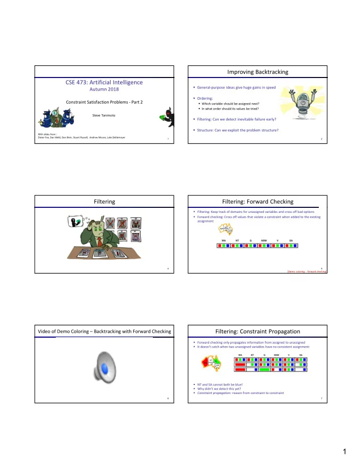
Improving Backtracking CSE 473: Artificial Intelligence General-purpose ideas give huge gains in speed Autumn 2018 Ordering: Constraint Satisfaction Problems - Part 2 Which variable should be assigned next? In what order should
Improving Backtracking CSE 473: Artificial Intelligence General-purpose ideas give huge gains in speed Autumn 2018 Ordering: Constraint Satisfaction Problems - Part 2 Which variable should be assigned next? In what order should its values be tried? Steve Tanimoto Filtering: Can we detect inevitable failure early? Structure: Can we exploit the problem structure? With slides from : Dieter Fox, Dan Weld, Dan Klein, Stuart Russell, Andrew Moore, Luke Zettlemoyer 1 2 Filtering Filtering: Forward Checking Filtering: Keep track of domains for unassigned variables and cross off bad options Forward checking: Cross off values that violate a constraint when added to the existing assignment NT Q WA SA NSW V 4 5 [Demo: coloring -- forward checking] Filtering: Constraint Propagation Video of Demo Coloring – Backtracking with Forward Checking Forward checking only propagates information from assigned to unassigned It doesn't catch when two unassigned variables have no consistent assignment: NT Q WA SA NSW V NT and SA cannot both be blue! Why didn’t we detect this yet? Constraint propagation: reason from constraint to constraint 6 7 1
Consistency of a Single Arc Arc Consistency of an Entire CSP A simple form of propagation makes sure all arcs are consistent: An arc X Y is consistent iff for every x in the tail there is some y in the head which could be assigned without violating a constraint NT Q NT WA Q SA WA NSW SA NSW V V Important: If X loses a value, neighbors of X need to be rechecked! Arc consistency detects failure earlier than forward checking Remember: Delete Can be run as a preprocessor or after each assignment Delete from the tail! from the tail! What’s the downside of enforcing arc consistency? Forward checking: Enforcing consistency of arcs pointing to each new assignment 8 9 AC-3 algorithm for Arc Consistency Limitations of Arc Consistency After enforcing arc consistency: Can have one solution left Can have multiple solutions left Can have no solutions left (and not know it) Arc consistency still runs What went Runtime: O(n 2 d 3 ), can be reduced to O(n 2 d 2 ) wrong here? inside a backtracking search! … but detecting all possible future problems is NP-hard – why? [Demo: coloring -- forward checking] 10 11 [Demo: CSP applet (made available by aispace.org) -- n-queens] [Demo: coloring -- arc consistency] K-Consistency K-Consistency Increasing degrees of consistency 1-Consistency (Node Consistency): Each single node’s domain has a value which meets that node’s unary constraints 2-Consistency (Arc Consistency): For each pair of nodes, any consistent assignment to one can be extended to the other K-Consistency: For each k nodes, any consistent assignment to k-1 can be extended to the k th node. Higher k more expensive to compute (You need to know the algorithm for k=2 case: arc consistency) 12 13 2
Strong K-Consistency Video of Demo Arc Consistency – CSP Applet – n Queens Strong k-consistency: also k-1, k-2, … 1 consistent Claim: strong n-consistency means we can solve without backtracking! Why? Choose any assignment to any variable Choose a new variable By 2-consistency, there is a choice consistent with the first Choose a new variable By 3-consistency, there is a choice consistent with the first 2 … Lots of middle ground between arc consistency and n-consistency! (e.g. k=3, called path consistency) 14 15 Video of Demo Coloring – Backtracking with Forward Checking – Video of Demo Coloring – Backtracking with Arc Consistency – Complex Graph Complex Graph 16 17 Ordering Ordering: Minimum Remaining Values Variable Ordering: Minimum remaining values (MRV): Choose the variable with the fewest legal left values in its domain Why min rather than max? Also called “most constrained variable” “Fail-fast” ordering 18 19 3
Ordering: Maximum Degree Ordering: Least Constraining Value Tie-breaker among MRV variables Value Ordering: Least Constraining Value Given a choice of variable, choose the least What is the very first state to color? (All have 3 values remaining.) constraining value Maximum degree heuristic: I.e., the one that rules out the fewest values in the remaining variables Choose the variable participating in the most constraints on remaining Note that it may take some computation to variables determine this! (E.g., rerunning filtering) Why least rather than most? Combining these ordering ideas makes Why most rather than fewest constraints? 1000 queens feasible 20 21 Rationale for MRV, MD, LCV Structure We want to enter the most promising branch, but we also want to detect failure quickly MRV+MD: Choose the variable that is most likely to cause failure It must be assigned at some point, so if it is doomed to fail, better to find out soon LCV: We hope our early value choices do not doom us to failure Choose the value that is most likely to succeed 22 23 Problem Structure Tree-Structured CSPs Extreme case: independent subproblems Example: Tasmania and mainland do not interact Independent subproblems are identifiable as connected components of constraint graph Suppose a graph of n variables can be broken into subproblems of only c variables: Worst-case solution cost is O((n/c)(d c )), linear in n Theorem: if the constraint graph has no loops, the CSP can be solved in O(n d 2 ) time E.g., n = 80, d = 2, c =20 Compare to general CSPs, where worst-case time is O(d n ) 2 80 = 4 billion years at 10 million nodes/sec (4)(2 20 ) = 0.4 seconds at 10 million nodes/sec This property also applies to probabilistic reasoning (later): an example of the relation between syntactic restrictions and the complexity of reasoning 24 25 4
Tree-Structured CSPs Tree-Structured CSPs Algorithm for tree-structured CSPs: Claim 1: After backward pass, all root-to-leaf arcs are consistent Order: Choose a root variable, order variables so that parents precede children Proof: Each X Y was made consistent at one point and Y’s domain could not have been reduced thereafter (because Y’s children were processed before Y) Claim 2: If root-to-leaf arcs are consistent, forward assignment will not backtrack Remove backward: For i = n : 2, apply RemoveInconsistent(Parent(X i ),X i ) Proof: Induction on position Assign forward: For i = 1 : n, assign X i consistently with Parent(X i ) Runtime: O(n d 2 ) (why?) Why doesn’t this algorithm work with cycles in the constraint graph? Note: we’ll see this basic idea again with Bayes’ nets 27 28 Improving Structure Nearly Tree-Structured CSPs Conditioning: instantiate a variable, prune its neighbors' domains Cutset conditioning: instantiate (in all ways) a set of variables such that the remaining constraint graph is a tree Cutset size c gives runtime O( (d c ) (n-c) d 2 ), very fast for small c 29 30 Cutset Conditioning Cutset Quiz Find the smallest cutset for the graph below. Choose a cutset SA Instantiate the cutset (all possible ways) SA SA SA Compute residual CSP for each assignment Solve the residual CSPs (tree structured) 31 32 5
Local Search for CSPs Iterative Algorithms for CSPs Local search methods typically work with “complete” states, i.e., all variables assigned To apply to CSPs: Take an assignment with unsatisfied constraints Operators reassign variable values No fringe! Live on the edge. Algorithm: While not solved, Variable selection: randomly select any conflicted variable Value selection: min-conflicts heuristic: Choose a value that violates the fewest constraints I.e., hill climb with h(n) = total number of violated constraints 34 35 Example: 4-Queens Performance of Min-Conflicts Given random initial state, can solve n-queens in almost constant time for arbitrary n with high probability (e.g., n = 10,000,000)! The same appears to be true for any randomly-generated CSP except in a narrow range of the ratio States: 4 queens in 4 columns (4 4 = 256 states) Operators: move queen in column Goal test: no attacks Evaluation: c(n) = number of attacks 36 39 [Demo: n-queens – iterative improvement (L5D1)] [Demo: coloring – iterative improvement] Summary: CSPs CSPs are a special kind of search problem: States are partial assignments Goal test defined by constraints Basic solution: backtracking search Speed-ups: Ordering Filtering Structure Iterative min-conflicts is often effective in practice 40 6
Recommend
More recommend
Explore More Topics
Stay informed with curated content and fresh updates.
