1 Gaussian Fun Facts Well add to these as we go along! First, - PDF document

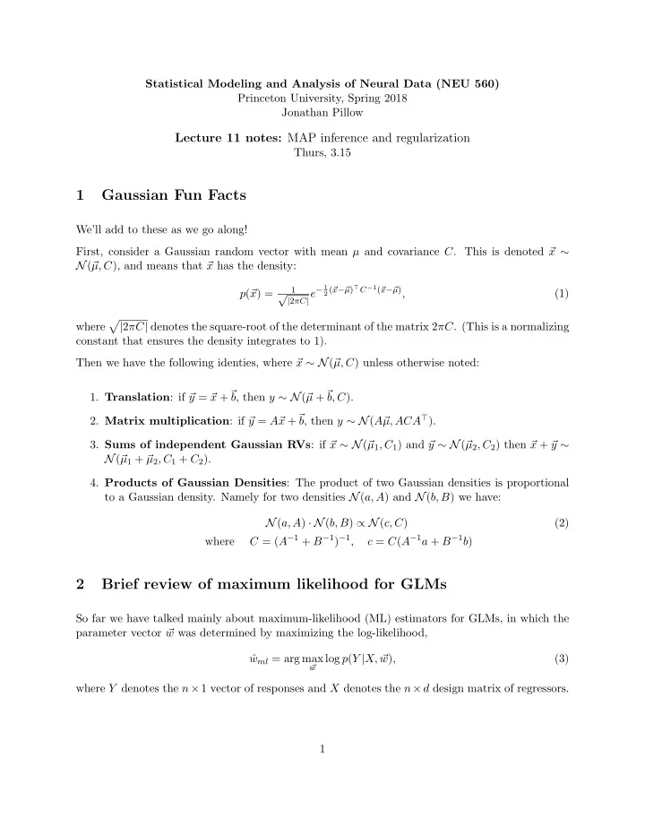
Statistical Modeling and Analysis of Neural Data (NEU 560) Princeton University, Spring 2018 Jonathan Pillow Lecture 11 notes: MAP inference and regularization Thurs, 3.15 1 Gaussian Fun Facts We’ll add to these as we go along! First, consider a Gaussian random vector with mean µ and covariance C . This is denoted � x ∼ N ( � µ, C ), and means that � x has the density: | 2 πC | e − 1 µ ) ⊤ C − 1 ( � 1 2 ( � x − � x − � µ ) , √ p ( � x ) = (1) � | 2 πC | denotes the square-root of the determinant of the matrix 2 πC . (This is a normalizing where constant that ensures the density integrates to 1). Then we have the following identies, where � x ∼ N ( � µ, C ) unless otherwise noted: x + � µ + � b , then y ∼ N ( � 1. Translation : if � y = � b, C ). x + � µ, ACA ⊤ ). 2. Matrix multiplication : if � y = A� b , then y ∼ N ( A� x ∼ N ( � y ∼ N ( � y ∼ 3. Sums of independent Gaussian RVs : if � µ 1 , C 1 ) and � µ 2 , C 2 ) then � x + � N ( � µ 1 + � µ 2 , C 1 + C 2 ). 4. Products of Gaussian Densities : The product of two Gaussian densities is proportional to a Gaussian density. Namely for two densities N ( a, A ) and N ( b, B ) we have: N ( a, A ) · N ( b, B ) ∝ N ( c, C ) (2) C = ( A − 1 + B − 1 ) − 1 , c = C ( A − 1 a + B − 1 b ) where 2 Brief review of maximum likelihood for GLMs So far we have talked mainly about maximum-likelihood (ML) estimators for GLMs, in which the parameter vector � w was determined by maximizing the log-likelihood, log p ( Y | X, � w ml = arg max ˆ w ) , (3) w � where Y denotes the n × 1 vector of responses and X denotes the n × d design matrix of regressors. 1

Linear Gaussian model: In the case of the “linear Gaussian GLM”, we had a closed form solution for the maximum-likelihood estimator. Here, the likelihood was given by a multi-variate normal distribution: w, σ 2 I ) , Y | X, � w ∼ N ( X � (4) where σ 2 denotes the variance of the (additive Gaussian) noise in Y . The maximum was given by w ml = ( X ⊤ X ) − 1 X ⊤ Y. ˆ (5) 3 Bayesian approach Today we will focus take a Bayesian approach and focus on the posterior distribution over � w given the data, which depends on a combination of the likelihood with a prior distribution . The posterior is given by Bayes rule: prior likelihood posterior � �� � � �� � P ( Y | X, � w | θ ) � �� � w ) P ( � P ( � w | Y, X, θ ) = . (6) P ( Y | X, θ ) � �� � “marginal likelihood” or “evidence” w | θ ) depends on a set of parameters θ that we will typically refer as hyperparameters . The prior p ( � These hyperparameters determine the shape (or strength) of the prior distribution. The term in the denominator, known as the marginal likelihood or evidence is a normalizing constant that does not depend on � w . Its purpose is simply to make sure that the posterior distribution � integrates to 1, that is, p ( � w | Y, X, θ ) d� w = 1. The denominator can therefore be seen as simply the integral of the stuff in the numerator: � � p ( Y | X, θ ) = p ( Y | X, � w | θ ) d� w | X, θ ) d� w ) p ( � w = p ( Y, � w, (7) where the rightmost expression expression shows that it is what we get by taking the joint distri- bution of Y and � w and marginalizing (integrating) over � w (hence the term “marginal likelihood”). 3.1 MAP inference / penalized maximum likelihood The maximum a posteriori (MAP) estimator corresponds to the maximum of the posterior: w map = arg max ˆ p ( � w | Y, X, θ ) . (8) w � Note that this is equivalent to maximizing the product of likelihood and prior, since the evidence (denominator in Bayes’ rule) does not involve � w and does not change the location of the maximum: � � w map = arg max ˆ p ( Y | X, � w ) P ( � w | θ ) = arg max log P ( Y | X, � w ) + log P ( � w | θ ) . (9) w � w � � �� � � �� � log-likelihood log-prior or ”penalty” 2

The last expression shows that the MAP estimator can be thought of as maximizing the log- likelihood plus a “penalty” given by the log-prior. This view motivates the terminology that refers to MAP estimation as “penalized log-likelihood”. 3.2 Common priors / penalties 1) L2 penalty - also known as “L2 shrinkage” or “ridge penalty” or “ridge prior” d � w || 2 = − 1 w ⊤ � penalty = − 1 w 2 i = − 1 2 λ || � 2 λ 2 λ� w (10) i =1 Corresponds to an independent Gaussian prior on the weights with variance θ = 1 λ : w ∼ N (0 , θI ) . � (11) The name “ridge prior” comes from the fact that the prior covariance matrix consists of a ridge of height θ along the main diagonal. To verify the equivalence: w ⊤ � w | θ ) = 1 log p ( � 2 θ � w + const (12) 2) L2 smoothing penalty - also known as “graph Laplacian”. d � penalty = − 1 ( w i − w i − 1 ) 2 2 λ (13) i =2 It turns out this operation (taking the sum squared pairwise difference between neighboring weights) can be embedded in the following matrix operation: i =2 ( w i − w i − 1 ) 2 = � sum d w ⊤ Γ � w (14) where Γ is the graph Laplacian defined by: Γ ii = degree, or # of neighbors of weight i Γ ij = − 1 if i and j are neighbors (15) Thus for example, for a “1-dimensional” weight vector � w = [ w 1 , w 2 , w 3 , w 4 ], we can compute the squared pairwise differences via: w || 2 = � w ⊤ D ⊤ D � w ⊤ Γ � || D � w = � w (16) where D is the pairwise-difference computing matrix:   − 1 1 0 0 D = 0 − 1 1 0 (17)   − 1 0 0 1 3

and Γ, the graph Laplacian is the tri-diagonal matrix:   1 − 1 − 1 2 − 1   D ⊤ D = Γ =  . (18)   − 1 2 − 1  − 1 1 Using this penalty is tantamount to a Gaussian prior given by: w ∼ N (0 , θ Γ − 1 ) � (19) although Γ, which is of rank d − 1 is not invertible, meaning that this is a “denerate” prior with infinite variance along the direction � w 1 = � w 2 = · · · = � w d . 3.3 MAP inference for linear-Gaussian model For the linear-Gaussian model we can compute the MAP estimate in closed form. We have the model now specified by w, σ 2 I ) , w ∼ N (0 , C ) Y | X, � � w ∼ N ( X � (20) where C is a prior covariance matrix (parametrized by θ ) and σ 2 is the variance of the additive noise in Y . The log-posterior is given by: wC − 1 � 1 w ) ⊤ ( Y − x� w ) − 1 log p ( Y | X, � w ) + log p ( � w | θ ) + const = 2 σ 2 ( Y − X � 2 � w + const w ⊤ C − 1 � = − 1 w ⊤ ( 1 σ 2 X ⊤ X ) � w − 1 w ( 1 σ 2 X ⊤ Y ) + const w − � 2 � 2 � w ⊤ ( 1 σ 2 X ⊤ X + C − 1 ) � σ 2 X ⊤ Y ) + const, = − 1 w ( 1 w − � 2 � (21) where const is a catch-all that collects terms that do not contain � w . Differentiating with respect to � w , setting to zero and solving gives: w map = ( X ⊤ X + σ 2 C − 1 ) − 1 X ⊤ Y ˆ (22) In the case of ridge regression, where prior covariance C = θI , this corresponds to w ridge = ( X ⊤ X + σ 2 θ I ) − 1 X ⊤ Y. ˆ (23) Thus the stimulus covariance X ⊤ X is added to a diagonal matrix with diagonal value σ 2 /θ , the ratio of noise variance to prior variance. The larger this value, the more the coefficients of � w map are shrunk towards zero. 4