1 Context The semantic gap Control-theoretical aspects Compilation - - PowerPoint PPT Presentation

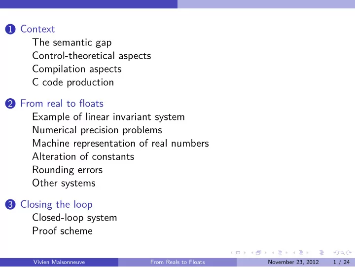
1 Context

The semantic gap Control-theoretical aspects Compilation aspects C code production

2 From real to floats

Example of linear invariant system Numerical precision problems Machine representation of real numbers Alteration of constants Rounding errors Other systems

3 Closing the loop

Closed-loop system Proof scheme

Vivien Maisonneuve From Reals to Floats November 23, 2012 1 / 24

From Physics to Interrupt Handlers: The Real to Float Step

Vivien Maisonneuve CRI, MINES ParisTech

Presentation at Toccata

November 23, 2012

Vivien Maisonneuve From Reals to Floats November 23, 2012 2 / 24

Context The semantic gap

Different levels of description

In control engineering, work on different levels to design and build a control system:

• Format/high-level aspects: system conception, modeling, possibly

proof.

• Concrete/low-level aspects: creation of an object implementing the

system. Quadricopter, DRONE Project, MINES ParisTech & ECP.

Vivien Maisonneuve From Reals to Floats November 23, 2012 3 / 24

Context The semantic gap

Formal aspect

model

• bject

System definition:

• Inputs: sensors [accelerometer, sonar. . . ] + references [operator

instructions]. Outputs: actions to act on environment [rotors rotation speed].

• Modeling in the form of equations to express relations between inputs

and outputs: differential equations/transfer functions between IOs.

Vivien Maisonneuve From Reals to Floats November 23, 2012 4 / 24

Context The semantic gap

Formal aspect

model

• bject

System definition:

• Inputs: sensors [accelerometer, sonar. . . ] + references [operator

instructions]. Outputs: actions to act on environment [rotors rotation speed].

• Modeling in the form of equations to express relations between inputs

and outputs: differential equations/transfer functions between IOs. System requirements:

• Stability conditions [bounded rotation speed].
• Pursuit of reference input [try to reach the ordered position].
• Perturbation rejection [wind].

Vivien Maisonneuve From Reals to Floats November 23, 2012 4 / 24

Context The semantic gap

Concrete aspect

model

• bject

Creation of a real object implementing the system.

• Electronic circuit that physically computes the transfer function.
• With a microcontroller: a small system with processor, memory,

I/O devices, that runs a program implementing the transfer function. [ATMEGA128 Frequency: 16 MHz RAM: 4 KB

• Prog. mem.: 128 KB]

Vivien Maisonneuve From Reals to Floats November 23, 2012 5 / 24

Context The semantic gap

Semantic gap

model C code µC code Antagonism:

• Abstract, mathematical model.
• Microcontroller code: program written in C, then compiled.

Long (thousands of LoC), low-level (elementary operations, hardware management, interruptions). Series of transformations to go from abstract model to microcontroller code.

Vivien Maisonneuve From Reals to Floats November 23, 2012 6 / 24

Context The semantic gap

Semantic gap

model C code µC code Antagonism:

• Abstract, mathematical model.
• Microcontroller code: program written in C, then compiled.

Series of transformations to go from abstract model to microcontroller code. Problem of proof transposition: Considering a model with correction proofs [stability], how to transpose down these proofs at the code level? Interest: formally check the code, not only the model. Difficulties: semantic gap, non-equivalent transformations (⇒ proofs must be checked).

Vivien Maisonneuve From Reals to Floats November 23, 2012 6 / 24

Context Control-theoretical aspects

Control-theoretical aspects

model pseudocode C code µC code Produce a pseudocode from the abstract model:

• Solve the model differential equation, get a transfer function.

(Laplace transform/Z transform, initial conditions problem.)

• If continuous-time model, discretization.

(Problems with sampling, execution times.) while transposing the proof. Usual problems in control engineering. Once done, discrete-time system with a loop on the transfer function ⇒ pseudocode [in MATLAB]. Proof: invariants on this code.

Vivien Maisonneuve From Reals to Floats November 23, 2012 7 / 24

Context Compilation aspects

Compilation aspects

model pseudocode C code µC code At the other end: compilation of C code to machine code. Risks of error:

• Important changes in the code: elementary operations, management
• f registers and of memory stack, instruction jumps.
• Possible optimizations.

Solutions:

• “Existing C compilers are reliable enough.”
• Proof-preserving compilation [Barthe].
• Certified compilation [CompCert].

Vivien Maisonneuve From Reals to Floats November 23, 2012 8 / 24

Context C code production

What’s between?

model pseudocode C code µC code Opener question. Several challenges:

1 High level mathematical operations series of elementary

instructions [matrices, sinus].

2 Real values machine words with limited precision. 3 On a microcontroller, data/events acquisition raises interruptions

(real-time answer, energy consumption) ⇒ particular code structure.

Vivien Maisonneuve From Reals to Floats November 23, 2012 9 / 24

From real to floats Example of linear invariant system

Example system

Very simple, open-loop, linear system [Feron]. Pseudocode:

Ac = [0.4990, -0.0500; 0.0100, 1.0000]; state matrix (matrice de dynamique) Bc = [1;0]; input matrix (matrice de commande) Cc = [564.48, 0];

• utput matrix (matrice d’observation)

Dc = -1280; feedthrough matrix (matrice d’action directe) xc = zeros(2,1); xc =

xc1

xc2

• ∈ R2: controller state

receive(y,2); receive(yd,3); y ∈ R : reference input; yd ∈ R : real position while 1 yc = max(min(y - yd,1),-1); yc ∈ [−1, 1] : bounded gap u = Cc*xc + Dc*yc; u ∈ R : action to be performed xc = Ac*xc + Bc*yc; send(u,1); send, receive: blocking, 2nd arg. is channel id receive(y,2); receive(yd,3); end

Vivien Maisonneuve From Reals to Floats November 23, 2012 10 / 24

From real to floats Example of linear invariant system

Lyapunov theory

(Lyapunov) stability: all reachable states xc start near an equilibrium point xe and stay in a neighborhood V of xe forever. Lyapunov theory: NSC on V . On linear systems, provided as an equation that can be solved with LMIs, generally as an ellipsoid. Here, show that xc =

• xc1

xc2

• belongs to the ellipse:

EP = {x ∈ R2 | xT · P · x ≤ 1}, P = 10−3

• 0, 6742

0, 0428 0, 0428 2, 4651

• .

xc ∈ EP ⇐ ⇒ 0.6742x2

c1 + 0.0856xc1xc2 + 2.4651x2 c2 ≤ 1000.

40 20 20 40 20 10 10 20

Vivien Maisonneuve From Reals to Floats November 23, 2012 11 / 24

From real to floats Example of linear invariant system

Stability proof

xc = zeros(2,1); xc ∈ EP receive(y,2); receive(yd,3); xc ∈ EP while 1 xc ∈ EP yc = max(min(y - yd,1),-1); xc ∈ EP, y2

c ≤ 1

xc

yc

• ∈ EQµ

| Qµ =

µP

02×1 01×2 1 − µ

• , µ = 0.9991

u = Cc*xc + Dc*yc;

xc

yc

• ∈ EQµ

xc = Ac*xc + Bc*yc; xc ∈ E˜

P

| ˜ P = Ac Bc

• · Q−1

µ

· Ac Bc

T −1

send(u,1); xc ∈ E˜

P

receive(y,2); xc ∈ E˜

P

receive(yd,3); xc ∈ E˜

P

xc ∈ EP end

Proof given as code invariants. Implication (weakening) if two consecutive invariants. Most of them easy to check, some depend on theorems. Last implication: E˜

P ⊆ EP

closes the loop. Validity relies on parameters Ac, Bc, Cc, Dc, µ: algebric or numerical verification needed.

Vivien Maisonneuve From Reals to Floats November 23, 2012 12 / 24

From real to floats Example of linear invariant system

Digression: with C instructions

High level mathematical operations series of scalar elementary instructions. Here, matrix operations are expanded: the instruction

xc

yc

• ∈ EQµ

xc = Ac*xc + Bc*yc; xc ∈ E˜

P

| ˜ P = Ac Bc

• · Q−1

µ

· Ac Bc

T −1

becomes:

xc

yc

• ∈ EQµ

xb[0] = xc[0]; xb: buffer xb[1] = xc[1]; xc[0] = Ac[0][0]*xb[0]+Ac[0][1]*xb[1]+yc; xc[1] = Ac[1][0]*xb[0]+Ac[1][1]*xb[1]; ???

Vivien Maisonneuve From Reals to Floats November 23, 2012 13 / 24

From real to floats Example of linear invariant system

Digression: with C instructions

High level mathematical operations series of scalar elementary instructions. Here, matrix operations are expanded: the instruction

xc

yc

• ∈ EQµ

xc = Ac*xc + Bc*yc; xc ∈ E˜

P

| ˜ P = Ac Bc

• · Q−1

µ

· Ac Bc

T −1

becomes:

xc

yc

• ∈ EQµ

xb[0] = xc[0]; xb: buffer xb[1] = xc[1]; xc[0] = Ac[0][0]*xb[0]+Ac[0][1]*xb[1]+yc; xc[1] = Ac[1][0]*xb[0]+Ac[1][1]*xb[1]; xc ∈ E˜

P

| ˜ P = Ac Bc

• · Q−1

µ

· Ac Bc

T −1

Same computation: output invariant can be found [Feron].

Vivien Maisonneuve From Reals to Floats November 23, 2012 13 / 24

From real to floats Numerical precision problems

Numerical precision problems

To produce C code: real numbers binary finite-length machine words (32 b. or 64 b.). ⇒ Loss in accuracy, two consequences:

1 Constant values are slightly altered. 2 Rounding errors during computations.

Vivien Maisonneuve From Reals to Floats November 23, 2012 14 / 24

From real to floats Machine representation of real numbers

Machine representation of real numbers

1 Floating point: IEEE 754.

Not usual on microcontrollers. number = sign × 2exponent+cst. offset × fraction Correct rounding for base operations: +, -, *, /. ⇒ If [bounds on] operands are known, not special, far enough from extremal values, then rounding error is bounded for +, -, * (not /).

2 Fixed point.

If operands are not special, far enough from extremal values, then rounding error is bounded for +, -, *.

3 Two integers.

Vivien Maisonneuve From Reals to Floats November 23, 2012 15 / 24

From real to floats Machine representation of real numbers

Machine representation of real numbers

1 Floating point. 2 Fixed point. 3 Two integers. Rational representation: numerator, denominator.

• Base behavior: +, -, *, / follow rational definition + fraction

simplification: p1 q1 + p2 q2 = simpl p1q2 + p2q1 q1q2

• , etc.

No rounding error. Problem: numerator value can easily exceed integer bounds.

• Approximated behavior to ensure bounded numerator.

Vivien Maisonneuve From Reals to Floats November 23, 2012 15 / 24

From real to floats Alteration of constants

Alteration of constants

With IEEE 754, 32 bits, constants

Ac = [0.4990, -0.0500; 0.0100, 1.0000]; Bc = [1;0]; Cc = [564.48, 0]; Dc = -1280;

become

Ac ≈ [0.49900001287460327 , -0.05000000074505806; 0.009999999776482582, 1.0000]; Bc ≈ [1;0]; Cc ≈ [564.47998046875, 0]; Dc ≈ -1280;

Vivien Maisonneuve From Reals to Floats November 23, 2012 16 / 24

From real to floats Alteration of constants

Effect on proof

xc = zeros(2,1); xc ∈ EP receive(y,2); receive(yd,3); xc ∈ EP while 1 xc ∈ EP yc = max(min(y - yd,1),-1); xc ∈ EP, y2

c ≤ 1

xc

yc

• ∈ EQµ

| Qµ =

µP

02×1 01×2 1 − µ

• , µ = 0.9991

u = Cc*xc + Dc*yc;

xc

yc

• ∈ EQµ

xc = Ac*xc + Bc*yc; xc ∈ E˜

P

| ˜ P = Ac Bc

• · Q−1

µ

· Ac Bc

T −1

send(u,1); xc ∈ E˜

P

receive(y,2); xc ∈ E˜

P

receive(yd,3); xc ∈ E˜

P

xc ∈ EP end

Rest of the code and proof sketch unchanged. ˜ P depends on Ac, Bc, Cc, Dc, is altered. ⇒ Check that E˜

P ⊆ EP still

holds.

Vivien Maisonneuve From Reals to Floats November 23, 2012 17 / 24

From real to floats Rounding errors

Rounding errors

With real numbers, the implication

xc

yc

• ∈ EQµ

xc = Ac*xc + Bc*yc; xc ∈ E˜

P

| ˜ P = Ac Bc

• · Q−1

µ

· Ac Bc

T −1

holds. With floats, + and * introduce rounding errors. As xc, yc belong to an ellipsoid, they are bounded so the rounding error on xc can be bounded by (e1, e2).

Vivien Maisonneuve From Reals to Floats November 23, 2012 18 / 24

From real to floats Rounding errors

Super-ellipsoid

Let E˜

F ⊃ E˜ P an ellipse s.t.

∀xc ∈ E˜

P, ∀x′ c ∈ R2, |x′ c1 − xc1| ≤ e1 ∧ |x′ c2 − xc2| ≤ e2 =

⇒ x′

c ∈ E˜ F

(∗) Then:

xc

yc

• ∈ EQµ

xc = Ac*xc + Bc*yc; xc ∈ E˜

F

E˜

F can be the smallest magnification of E˜ P s.t. (∗)

holds. Can be computed, whatever number of dimensions.

Vivien Maisonneuve From Reals to Floats November 23, 2012 19 / 24

From real to floats Rounding errors

Effect on proof

xc = zeros(2,1); xc ∈ EP receive(y,2); receive(yd,3); xc ∈ EP while 1 xc ∈ EP yc = max(min(y - yd,1),-1); xc ∈ EP, y2

c ≤ 1

xc

yc

• ∈ EQµ

| Qµ =

µP

02×1 01×2 1 − µ

• , µ = 0.9991

u = Cc*xc + Dc*yc;

xc

yc

• ∈ EQµ

xc = Ac*xc + Bc*yc; xc ∈ E˜

F

send(u,1); xc ∈ E˜

F

receive(y,2); xc ∈ E˜

F

receive(yd,3); xc ∈ E˜

F

xc ∈ EP end

Replace E˜

P by E˜ F in proof

sketch. ⇒ Check that E˜

F ⊆ EP

holds. Here it works: system stable with floats .

Vivien Maisonneuve From Reals to Floats November 23, 2012 20 / 24

From real to floats Other systems

Other functions

Elementary operations +, * are sufficient for linear, invariant systems. The method applies if the proof sketch fits: no tight assumptions, complex

• perations on weakened invariants.

1-var, differentiable, periodic functions can be computed

• with an abacus and a polyhedral interpolation function
• with a polyhedral approximation

with a bounded error (sin, cos). Idem for 1-var, differentiable functions restricted to a finite range. OK if proof ensures the operand is bounded to the range.

Vivien Maisonneuve From Reals to Floats November 23, 2012 21 / 24

Closing the loop Closed-loop system

Closing the loop

Modeling the result of the effects of the action on the environment, with feedback. Design: here, two parallel, synchronized programs: controller + plant (abstract).

Ac = [0.4990, -0.0500; 0.0100, 1.0000]; Ap = [1.000, 0.0100; -0.0100, 1.000]; Bc = [1;0]; Bp = [0.00005; 0.01]; Cc = [564.48, 0]; Cp = [1, 0]; Dc = -1280; xc = zeros(2,1); receive(y,2); receive(yd,3); while 1 while (1) yc = max(min(y - yd,1),-1); yp = Cp * xp; u = Cc*xc + Dc*yc; send(yp,2); xc = Ac*xc + Bc*yc; receive(up,1); send(u,1); xp = Ap * xp + Bp * up; receive(y,2); end receive(yd,3); end

System is not linear.

Vivien Maisonneuve From Reals to Floats November 23, 2012 22 / 24

Closing the loop Proof scheme

Proving the system

Lyapunov stability: global state (xc, xp) in some ellipsoid EP. ⇒ + Boundedness of variables in physical system. Difficulties:

• Non-linearity issues: trickier to find a suitable EP, post-condition to

yc definition. Usual case here, has been dealt.

• Handling concurrency in invariants: switch between system and plant

analysis.

Vivien Maisonneuve From Reals to Floats November 23, 2012 23 / 24

Closing the loop Proof scheme

Proving the system

Ac = [0.4990, -0.0500; 0.0100, 1.0000]; Ap = [1.000, 0.0100; -0.0100, 1.000]; Bc = [1;0]; Bp = [0.00005; 0.01]; Cc = [564.48, 0]; Cp = [1, 0]; Dc = -1280; xc = zeros(2,1); receive(y,2); receive(yd,3); while 1 while (1) yc = max(min(y - yd,1),-1); yp = Cp * xp; u = Cc*xc + Dc*yc; send(yp,2); xc = Ac*xc + Bc*yc; receive(up,1); send(u,1); xp = Ap * xp + Bp * up; receive(y,2); end receive(yd,3); end

Vivien Maisonneuve From Reals to Floats November 23, 2012 23 / 24

Closing the loop Proof scheme

Proving the system

Lyapunov stability: global state (xc, xp) in some ellipsoid EP. ⇒ + Boundedness of variables in physical system. Difficulties:

• Non-linearity issues: trickier to find a suitable EP, post-condition to

yc definition. Usual case here, has been dealt.

• Handling concurrency in invariants: switch between system and plant

analysis.

• Invariants of greater dimension: cannot test algebraically invariant

inclusion, fails with floats.

• C code with interrupts.

SIGNAL(2) SIGNAL(3) while(1) { y = ... yd = ... sleep(); ... ... }

Vivien Maisonneuve From Reals to Floats November 23, 2012 23 / 24

Closing the loop Proof scheme

From Physics to Interrupt Handlers: The Real to Float Step

Vivien Maisonneuve CRI, MINES ParisTech

Presentation at Toccata

November 23, 2012

Vivien Maisonneuve From Reals to Floats November 23, 2012 24 / 24