Xavier Pennec Asclepios team, INRIA Sophia- Antipolis Mediterrane, - PowerPoint PPT Presentation

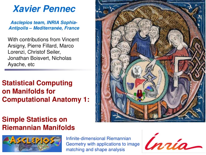
Xavier Pennec Asclepios team, INRIA Sophia- Antipolis – Mediterranée, France With contributions from Vincent Arsigny, Pierre Fillard, Marco Lorenzi, Christof Seiler, Jonathan Boisvert, Nicholas Ayache, etc Statistical Computing on Manifolds for Computational Anatomy 1: Simple Statistics on Riemannian Manifolds Infinite-dimensional Riemannian Geometry with applications to image matching and shape analysis

Science that studies the structure and the relationship in Anatomy space of different organs and tissues in living systems [Hachette Dictionary] 2007 Visible Human Project, NLM, 1996-2000 Voxel-Man, U. Hambourg, 2001 1st cerebral atlas, Vesale, 1543 Talairach & Tournoux, 1988 Paré, 1585 1990-2000: 17-20e century: Antiquity • Explosion of imaging Renaissance: • Animal models • Anatomo-physiology • Dissection, surgery • Computer atlases • Microscopy, histology • Philosophical physiology • Descriptive anatomy • Brain decade Vésale (1514-1564) Sylvius (1614-1672) Gall (1758-1828) : Phrenology Galien (131-201) Paré (1509-1590) Willis (1621-1675) Talairach (1911-2007) Revolution of observation means (1988-2007) : From dissection to in-vivo in-situ imaging  From representative individual to population  From descriptive atlases to interactive and generative models (simulation)  X. Pennec - ESI - Shapes, Feb 10-13 2015 2

Computational Anatomy Design Mathematical Methods and Algorithms to Model and Analyze the Anatomy  Statistics of organ shapes across species, populations, diseases…  Model organ development across time (heart- beat, growth, ageing, ages…)  To understand and to model how life is functioning Classify structural deviations ( taxonomy ), Relate anatomy and function   To detect, understand and correct dysfunctions From generic (atlas-based) to patients-specific models   Very active topic in medical image analysis Keyword of Medic Image Computing and Computer Assisted Intervention (MICCAI)  X. Pennec - ESI - Shapes, Feb 10-13 2015 3

Statistical Analysis of Geometric Features Noisy Geometric Measures  Tensors, covariance matrices  Curves, tracts  Surfaces  Transformations  Rigid, affine, locally affine, diffeomorphisms Goal:  Deal with noise consistently on these non-Euclidean manifolds  A consistent statistical (and computing) framework X. Pennec - ESI - Shapes, Feb 10-13 2015 5

Morphometry through Deformations Atlas  1  5 Patient 1 Patient 5  4  3  2 Patient 4 Patient 3 Patient 2 Measure of deformation [D’Arcy Thompson 1917, Grenander & Miller]  Observation = “random” deformation of a reference template  Reference template = Mean (atlas)  Shape variability encoded by the deformations Statistics on groups of transformations (Lie groups, diffeomorphism)? Consistency with group operations (non commutative)? X. Pennec - ESI - Shapes, Feb 10-13 2015 6

Methods of computational anatomy Remodeling of the right ventricle of the heart in tetralogy of Fallot  Mean shape  Shape variability  Correlation with clinical variables  Predicting remodeling effect Shape of RV in 18 patients X. Pennec - ESI - Shapes, Feb 10-13 2015 7

Longitudinal deformation analysis Dynamic obervations time Patient A ? ? Template Patient B How to transport longitudinal deformation across subjects? What are the convenient mathematical settings? X. Pennec - ESI - Shapes, Feb 10-13 2015 8

Statistical Computing on Manifolds for Computational Anatomy Simple Statistics on Riemannian Manifolds Manifold-Valued Image Processing Metric and Affine Geometric Settings for Lie Groups Analysis of Longitudinal Deformations X. Pennec - ESI - Shapes, Feb 10-13 2015 9

Statistical Computing on Manifolds for Computational Anatomy Simple Statistics on Riemannian Manifolds  Introduction to computational anatomy  The Riemannian manifold computational structure  Simple statistics on Riemannian manifolds  Applications to the spine shape and registration accuracy Manifold-Valued Image Processing Metric and Affine Geometric Settings for Lie Groups Analysis of Longitudinal Deformations X. Pennec - ESI - Shapes, Feb 10-13 2015 10

Basic probabilities and statistics Measure: random vector x of pdf ( z ) p x Σ ( x ) Approximation: ~ , x xx    • Mean: x E( ) . ( ). z p z dz x x       • Covariance: T E ( x ).( x ) x x xx Propagation:     T   h h    Σ ( ) x , . . h ~ h   y x   xx x   x Noise model: additive, Gaussian... Principal component analysis  2 Statistical distance: Mahalanobis and X. Pennec - ESI - Shapes, Feb 10-13 2015 11

Differentiable manifolds Définition:  Locally Euclidean Topological space which can be globally curved  Same dimension + differential regularity Simple Examples  Sphere  Saddle (hyperbolic space)  Surface in 3D space And less simple ones  Projective spaces  Rotations of R 3 : SO 3 ~ P 3  Rigid, affine Transformation  Diffeomorphisms X. Pennec - ESI - Shapes, Feb 10-13 2015 12

Differentiable manifolds Computing in a a manifold  Extrinsic  Embedding in ℝ 𝑜  Intrinsic  Coordinates : charts  Atlas = consistent set of charts  Measuring?  Volumes (surfaces)  Lengths  Straight lines X. Pennec - ESI - Shapes, Feb 10-13 2015 13

Measuring extrinsic distances Basic tool: the scalar product  ,  t v w v w • Norm of a vector    , v v v • Angle between vectors    , cos( ) v w v w g (t) • Length of a curve v w  g  g  ( ) || ( ) || L t dt p X. Pennec - ESI - Shapes, Feb 10-13 2015 14

Measuring extrinsic distances Basic tool: the scalar product  ,     t t , ( ) v v w w v v w G p w p • Norm of a vector    , v v v Bernhard Riemann p 1826-1866 p • Angle between vectors Bernhard Riemann     1826-1866 , cos( ) v w v w p p p • Length of a curve  g  g  ( ) || ( ) || t L t dt g ( ) X. Pennec - ESI - Shapes, Feb 10-13 2015 15

Riemannian manifolds Basic tool: the scalar product    t , ( ) v w v G p w p Bernhard Riemann 1826-1866 • Geodesic between 2 points Bernhard Riemann 1826-1866 • Shortest path • Calculus of variations (E.L.) : • Length of a curve 2 nd order differential equation  g  g (specifies acceleration)  ( ) || ( ) || t L t dt g ( ) • Free parameters: initial speed and starting point X. Pennec - ESI - Shapes, Feb 10-13 2015 16

Bases of Algorithms in Riemannian Manifolds Exponential map (Normal coordinate system):  Exp x = geodesic shooting parameterized by the initial tangent  Log x = unfolding the manifold in the tangent space along geodesics  Geodesics = straight lines with Euclidean distance  Local  global domain: star-shaped, limited by the cut-locus  Covers all the manifold if geodesically complete Reformulate algorithms with exp x and log x Vector -> Bi-point (no more equivalence classes) Operation Euclidean space Riemannian    Subtraction ( y ) xy y x xy Log x    ( xy ) y Exp Addition y x xy x    dist ( , ) dist ( , ) x y y x Distance x y xy x         ( ) ( ( )) x x C x x Exp C x Gradient descent     t x t t t t t X. Pennec - ESI - Shapes, Feb 10-13 2015 17

Statistical Computing on Manifolds for Computational Anatomy Simple Statistics on Riemannian Manifolds  Introduction to computational anatomy  The Riemannian manifold computational structure  Simple statistics on Riemannian manifolds  Applications to the spine shape and registration accuracy Manifold-Valued Image Processing Metric and Affine Geometric Settings for Lie Groups Analysis of Longitudinal Deformations X. Pennec - ESI - Shapes, Feb 10-13 2015 21

Random variable in a Riemannian Manifold Intrinsic pdf of x  For every set H 𝑄 𝐲 ∈ 𝐼 = 𝑞 𝑧 𝑒𝑁(𝑧) 𝐼  Lebesgue’s measure  Uniform Riemannian Mesure 𝑒𝑁 𝑧 = det 𝐻 𝑧 𝑒𝑧 Expectation of an observable in M  𝑭 𝐲 𝜚 = 𝜚 𝑧 𝑞 𝑧 𝑒𝑁 𝑧 𝑁  𝜚 = 𝑒𝑗𝑡𝑢 2 (variance) : 𝑭 𝐲 𝑒𝑗𝑡𝑢 . , 𝑧 2 = 𝑒𝑗𝑡𝑢 𝑧, 𝑨 2 𝑞 𝑨 𝑒𝑁(𝑨) 𝑁  𝜚 = log 𝑞 (information) : 𝑭 𝐲 log 𝑞 = 𝑞 𝑧 log (𝑞 𝑧 )𝑒𝑁 𝑧 𝑁  𝜚 = 𝑦 (mean) : 𝑭 𝐲 𝐲 = 𝑧 𝑞 𝑧 𝑒𝑁 𝑧 𝑁 X. Pennec - ESI - Shapes, Feb 10-13 2015 22