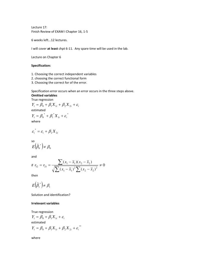

Lecture 17: Finish Review of EXAM I Chapter 16, 1 ‐ 5 6 weeks left...12 lectures. I will cover at least chpt 6 ‐ 11. Any spare time will be used in the lab. Lecture on Chapter 6 Specification: 1. Choosing the correct independent variables 2. choosing the correct functional form 3. Choosing the correct for of the error. Specification error occurs when an error occurs in the three steps above. Omitted variables True regression Y X X i 0 1 1 i 2 2 i i estimated * * * Y X i 0 1 1 i i where * X 2 i i 2 i so ˆ * E 0 0 and ( x x )( x x ) 1 1 2 2 r r 0 if 12 21 2 2 ( x x ) ( x x ) 1 1 2 2 then ˆ * E 1 1 Solution and identification? Irrelevant variables True regression Y X i 0 1 1 i i estimated * * Y X X i 0 1 1 i 2 2 i i where
* * X 2 i i 2 i Four Important Specification Criteria 1. Theory 2. T ‐ test 3. Rbar squared 4. Bias (do variables coefficients change significantly when variables are added) Specification Searches Data Mining http://www.absoluteastronomy.com/topics/Testing_hypotheses_suggested_by_the_data Stepwise regressions http://www.stata.com/support/faqs/stat/stepwise.html Sequential searches Using T ‐ tests to choose included variables Scanning and Sensitivity analysis So how do we choose a model?
Lecture 18: October 31 Lagged independent variables Ramsey Regression Specification Error Test (RESET) A test for misspecification and sometimes, rather mistakenly referred t as a test for omitted variables Using OLS estimate ˆ ˆ ˆ ˆ Y X X eq 1 i 0 1 1 i 2 2 i ˆ ˆ ˆ 2 3 4 Y , Y , Y then generate i i i re ‐ estimate the original equation augmenting it with the polynomials of the fitted values. ˆ ˆ ˆ 2 3 4 Y X X Y Y Y eq 2 i i i 0 1 1 i 2 2 i 3 4 5 i ( RSS RSS ) M m F RSS ( n ( k 1 )) where RSS_m is from eq 1 and RSS is from eq 2. Ramsey’s Regression Specification Error Test (RESET) http://faculty.chass.ncsu.edu/garson/PA765/assumpt.htm � Ramsey's RESET test (regression specification error test). Ramsey's general test of specification error of functional form is an F test of differences of R2 under linear versus nonlinear assumptions. It is commonly used in time series analysis to test whether power transforms need to be added to the model. For a linear model which is properly specified in functional form, nonlinear transforms of the fitted values should not be useful in predicting the dependent variable. While STATA and some packages label the RESET test as a test to see if there are "no omitted variables," it is a linearity test, not a general specification test. It tests if any nonlinear transforms of the specified independent variables have been omitted. It does not test whether other relevant linear or nonlinear variables have been omitted. 1. Run the regression to obtain Ro2, the original multiple correlation. 2. Save the predicted values (Y's). 3. Re ‐ run the regression using power functions of the predicted values (ex., their squares and cubes) as additional independents for the Ramsey RESET test of functional form where testing that none of the independents is nonlinearly related to the dependent. Alternatively, re ‐ run the regression using power functions of the independent variables to test them individually. 4. Obtain Rn2, the new multiple correlation. 5. Apply the F test, where F = ( Rn2 ‐ Ro2)/[(1 ‐ Rn2)/(n ‐ p)], where n is sample size and p is the number of parameters in the new model. 6. Interpret F: For an adequately specified model, F should be non ‐ significant. Apparently some stats programs have rounding errors/computational problems that appear as multicollinearity. http://en.wikipedia.org/wiki/Multicollinearity
4) Mean ‐ center the predictor variables. Mathematically this has no effect on the results from a regression. However, it can be useful in overcoming problems arising from rounding and other computational steps if a carefully designed computer program is not used. But really, it shouldn't truly matter. http://www.bauer.uh.edu/jhess/papers/JMRMeanCenterPaper.pdf But now that I do some digging I see that stata actually does this normalization as well, before taking the powers. http://www.stata.com/statalist/archive/2004 ‐ 06/msg00264.html Akaike Information Criterion (AIC) Minimize AIC=Log(RSS/n)+2(K+1)/n Schwarz Criterion, or Schwarz Bayesian Criterion (SC, SBC) Minimize SBC=Log(RSS/n)+Log(n)(K+1)/n
Lecture 19: November 4 The use and interpretation of the constant term Don’t do it. There is an inherent identification problem, as the constant includes the true constant, means of omitted variables, and Alternative functional forms Linear Form Y X X i 0 1 1 i 2 2 i i Double log form ln Y ln X ln X i 0 1 1 i 2 2 i i Semi ‐ log form Log – Lin ln Y X X i 0 1 1 i 2 2 i i Lin ‐ Log Y ln X ln X i 0 1 1 i 2 2 i i Polynomial functional form 2 Y X X i 0 1 1 i 2 i 1 i Inverse functional Form Y ( 1 / X ) X i 0 1 1 i 2 2 i i Be sure to appropriately interpret the marginal effects. Elasticities, percentage changes etc. Never take the log of a dummy variable. Almost always take the log of a dollar value. Problems with incorrect functional form. Some pictures of alternative forms.
Level 160.0 140.0 120.0 100.0 80.0 60.0 40.0 20.0 0.0 LN 6.0 5.0 4.0 3.0 2.0 1.0 0.0
Rsquared are difficult to compare when transformed Incorrect functional forms Estimate
Lecture 20 :November 7 Using dummy variables Intercept dummy Y X X i 0 1 1 i 2 2 i i Where: Y is salary X1 is a dummy variable for male x2=1 for male, 0 for female. X2 is marketability . r egr ess sal ar y m al e m ar ket c Sour ce SS df M S Num ber of obs = 51 514 F( 2, 511) = 8 85. 8 5. 80 M odel 2. 0 2. 071 711e+ 1e+10 10 2 2 1 1. 03 . 0356e 56e+10 +10 Pr ob > F = 0. 0. 000 0000 Resi dual 6. 1 6. 167 676e+ 6e+10 10 5 511 120 120696 696838 838 R- squar ed = 0. 0. 251 2514 Adj R- squar ed = 0. 0. 248 2485 Tot al 8. 2 8. 238 387e+ 7e+10 10 5 513 160 160599 599133 133 Root M SE = 1 1098 0986 sal ar y Coef . St d. Er r . t P>| t | [ 95% Conf . I nt er val ] m al e 87 8708 08. 42 . 423 3 11 1139 39. 41 . 411 1 7. 6 7. 64 4 0 0. 00 . 000 0 64 6469. 69. 917 917 1 1094 0946. 9 6. 93 m ar ket c 2 29972. 72. 6 6 33 3301 01. 76 . 766 6 9. 0 9. 08 8 0 0. 00 . 000 0 23 23485 485. 89 . 89 364 36459. 59. 3 _cons 44 4432 324. 0 4. 09 9 98 983. 3. 353 3533 3 4 45. 0 5. 07 7 0 0. 00 . 000 0 42 42392 392. 17 . 17 4 4625 6256 As a follow up from the previous section, I re ‐ run the regression using the log of salary as the dependent variable. Notice a few things, the R ‐ squared is different, but remember that should not be used to decide on models as the dependent variable has a different total sum of squares. Do notice that the coefficient on male is quantitatively different. Now its interpretation is the effect of being male not on salary, but the log of salary, or the percentage change. So being male means a 7.6% increase in salary relative to females holding market constant, but not other excluded/omitted variables.
Recommend
More recommend